|
|
(2.2) |
Karl Skretting, University of Stavanger.
| Contents on this page: | Relevant papers and links to other pages: |
|---|---|
|
|
Dictionary Learning is a topic in the Signal Processing area,
the dictionary is usually used for Sparse Representation or Approximation of signals.
A dictionary is a collection of atoms, here the atoms are real column vectors of length N.
A finite dictionary of K atoms can be represented
as a matrix D of size NxK.
In a Sparse Representation a vector x is represented or approximated as a linear
combination of some few of the dictionary atoms.
The approximation xa can be written as
xa = D wwhere w is a vector containing the coefficients and
most of the entries in w are zero.
Dictionary Learning is the problem of finding a dictionary such that the approximations of
many vectors, the training set, are as good as possible given a sparseness criterion on the coefficients,
i.e. allowing only a small number of non-zero coefficients for each approximation.
This page describes some experiments done on Dictionary Learning. The complete theory of dictionary learning is not told here, only a brief overview (of some parts) is given in section 3. and some links to relevant papers are included on the upper right part of this page. Section 4 presents the results of the experiments used in the RLS-DLA paper, and section 6 also includes the files needed to redo the experiments.
In Matlab version 2012a Matching Pursuit algorithms are included in the wavelet toolbox, see Wavelet Toolbox User Guide.
Let the dictionary D be represented as a real matrix of size
NxK and K>N.
Given a test vector x of size Nx1,
it can be approximated by a linear combination of dictionary atoms,
the column vectors of D are often called atoms in a sparse approximation context.
Denoting the atoms as d1, d2, ... , dK,
one example of a sparse approximation is
xa = w(1)d1 + w(4)d4 + w(7)d7 + w(9)d9, |
x = xa + r |
(2.1) |
where four of the atoms have been used here. r is the representation error.
The elements w(i) (where i is 1, 4, 7 and 9 in this example)
are the coefficients in the representation.
Collecting the coefficients into a vector w
the approximation xa can be written as:
xa = D w, and the representation error can be written as
: r = x - xa = x - D w.
If most of the entries in w are zero this is a sparse representation,
the number of non-zero coefficients is s and the sparsness factor is s/N.
The problem of finding w is the sparse approximation problem;
minimize ||x - D w|| subject to number of non-zeros in w smaller or equal to s.
A common way to write this problem is
|
|
(2.2) |
As γ increases the solution is getting more dense.
The problem with p=0 is NP-hard.
Good, but not necessarily optimal, solutions can be found by matching pursuit algorithms,
for example the order recursive matching pursuit (ORMP) algorithm.
The problem with p=1 is easier, the LARS algorithm is effective for solving this problem.
Both ORMP and LARS find w in a greedy way, starting with an all zero vector in w,
which is the solution when γ is close to zero, then the algorithms
add one and one vector based on some rules given by the algorithm.
For the LARS algorithm this corresponds to all the solutions to Eq. 2.2 above
with p=1 and γ gradually increases.
For both ORMP and LARS there must be a stopping criterium,
the algorithm returns when the stopping criterion is reached.
This can be that the 0-norm (number of non-zeros) the 1-norm (sum of absolute values) or
that the error (sum of squared errors) have reached a predefined limit.
We should note that both LARS and ORMP implementations often are more effective when a fixed dictionary
D can be used to find the solutions for several signal vectors at once.
The function sparseapprox.m is a general sparse approximation function which contains several methods, and also acts as interface to external functions. The available methods can be devided into four groups:
mpv2
java package (by K. Skretting) is available then sparseapprox.m can be used to access
some of the matching pursuit variants implemented there:
javaMP, javaOMP, javaORMP and javaPS, the
last one is partial search as described in the
Partial Search paper.
This paper also describes the details of and difference between OMP and ORMP.
A test of the sparseapprox.m function is done by ex300.m.
The dictionary and the data in the mat-files included in the table at the bottom of this
page is used and sparse approximations are found using several methods avaliable from sparseapprox.m.
The results are presented in a table, parts of that table is shown here.
Time is given in seconds (for the 4000 sparse approximations done), SNR is signal to noise ratio,
w0 is average 0-norm for the coefficient, i.e. the first term in Eq. 2.2 with p=0,
w1 is average 1-norm for the coefficient, i.e. the first term in Eq. 2.2 with p=1,
and r2 is average 2-norm for the errors, i.e. the second term in Eq. 2.2.
Here pinv, linprog and FOCUSS are followed by thresholding
and the coefficients are adjusted by an orthogonal projection onto the column space of the seleceted columns.
We can note that there is a pattern in the matching pursuit algorithms, as the error is
decreased, from MP to OMP to ORMP to PS(10) to PS(250), the 1-norm of the coefficients is increased.
| Method | Time | SNR | w0 | w1 | r2 |
|---|---|---|---|---|---|
| pinv | 0.59 | 4.88 | 4 | 14.59 | 6.29 |
| linprog | 58.99 | 9.94 | 4 | 16.43 | 3.75 |
| FOCUSS | 29.68 | 16.95 | 3.9 | 14.62 | 1.79 |
| mexLasso | 0.07 | 11.90 | 3.96 | 10.28 | 3.13 |
| javaMP | 0.49 | 16.89 | 4 | 16.19 | 1.81 |
| OMP | 8.12 | 17.86 | 4 | 16.86 | 1.61 |
| javaOMP | 0.56 | 17.86 | 4 | 16.86 | 1.61 |
| ORMP | 8.53 | 18.27 | 4 | 18.12 | 1.54 |
| javaORMP | 0.30 | 18.27 | 4 | 18.12 | 1.54 |
| mexOMP | 0.05 | 18.27 | 4 | 18.12 | 1.54 |
| Partial Search (10) | 0.55 | 18.79 | 4 | 20.21 | 1.45 |
| Partial Search (250) | 3.95 | 19.00 | 4 | 23.17 | 1.42 |
The Shift Invariant Dictionary (SID) structure and the algorithm for sparse approximation using SID
were both presented in the Scandinavian Conference on Image Analysis, Tromsø Norway, June 12-14 2017,
paper available in proceedings part 1, page 362-373, or this link
SCIA 2017 paper.
In Matlab the SID can be in initialized by initSID.m,
or initSID2D.m for the 2D case.
The SID can be visualized by plotSID.m,
or plotSID2D.m for the 2D case. Example:
Qm = [35,26,20,10,9]; Pm = [5,2,2,1,1]; sid = initSID(Qm,Pm); plotSID(sid, 1);
D = makeSIDmatrix(sid,50); clf; spy(D); % make D a 50x116 matrix in this case
The Matlab sparse approximation implementations use several m-files and one mex-file (I hope I got it all here).
Some needed and helpful files are: For expanding the compact SID representation into sparse dictionary matrix you may use
makeSIDmatrix.m and makeSID2Dmatrix.m.
For matrix multiplication (using the compact SID representation) three functions are made multSID.m,
multSIDt.m and multSID2D.m.
The sparse approximation (Basic Matching Pursuit) is done by saSIDbmp2.m
and it needs a mex-file for fast execution, saSIDbmp_mex.c.
Orthogonal MP variants are available for both the 1D and the 2D variant,
saSIDomp.m and saSID2Domp.m,
both use sparseapprox.m to do the actual work.
Example (sid as above):
N = 50000; sf = 1/8; s = floor(N*sf);

y = filter(1,[1,-0.98],randn(N,1)); syy = sum( y.^2 );  % AR(1) signal

wbmp = saSIDbmp2(y, sid, s);

yr = multSID(sid, wbmp, N);

see = sum( (y-yr).^2 ); snrbmp = 10*log10(syy/see);

womp = saSIDomp(y, sid, wbmp); % improve wbmp

yr = multSID(sid, womp, N);

see = sum( (y-yr).^2 ); snromp = 10*log10(syy/see);
A common setup for the dictionary learning problem starts with access to a training set,
a collection of training vectors, each of lenght N.
This training set may be finite, then the training vectors are usually collected
as columns in a matrix X of size NxL, or it may be infinite.
For the finite case the aim of dictionary learning is to find both a dictionary, D of size NxK, and a corresponding coefficient matrix W of size KxL such that the
representation error, R=X-DW, is minimized and W fulfill some sparseness criterion.
The dictionary learning problem can be formulated as an optimization problem with respect to W and D, with γ and p are as in Eq. 2.2 we may put it as
 |
(3.1) |
The Matlab function dlfun.m,
attached in the end of this page, can be used for MOD, K-SVD, ODL or RLS-DLA.
It is entirely coded in Matlab, except that the sparse approximation, done by sparseapprox.m,
may call java or mex functions if this is specified.
The help text of dlfun.m gives some examples for how to use it.
Note that this function is slow as sparse approximation is done for only one vector each time,
an improvement (in speed) would be to do all the sparse approximations in one function call for
MOD and K-SVD, or to use a mini-batch approach like LS-DLA for ODL and RLS-DLA.
However, processing one training vector at a time may give better control of the algorithm
and gives more precise information in error messages and exception handling.
Method of Optimized Directions (MOD), or iterative least squares dictionary learning algorithms (ILS-DLA)
as the family of MOD-algorithms (many variants exist) may be denoted, can be used for a finite learning set,
X of size NxL,
and with sparseness defined by either 0-norm (number of non-zero coefficient is limited)
or 1-norm (sum of absolute values of coefficient is limited), i.e. p=0 or p=1.
The optimization problem of Eq. 3.1 is divided into two (or three) parts iteratively solved
D fixed find W,
this gives L independent problems as in Eq. 2.2, and
W fixed find D using the least squares solution:
D = (XWT)(WWT)-1 = BA-1.
It is convenient to define the matrices B=XWT and A=WWT.
D, i.e. scale each column vector (atom) of D to unit norm.
Part 3 may be skipped if D is almost normalized and the l0-sparseness is used.
Part 1 is computationally most demanding, and with this setup there will be a lot of computational effort
between each dictionary update, slowing down the learning process. This is especially true with large training sets.
Some minor adjustments can be done to improve the learning speed for large (and also medium sized) training sets, this variant can be denoted as the large-MOD variant.
The training set is (randomly) divided into M (equal sized) subsets, the subsets are denoted Xm for m=1 to M.
Now, for each iteration we only use one, some few, (or perhaps almost all) of the subsets of training vectors in part 1 above.
Which subsets to use may be randomly chosen, or the subsets which has been unused for the longest time can be selected.
Anyway, finding new coefficients for only a part of the total number of training vectors reduces the time used.
In part 2 the matrices A and B are calculated by adding products of training vector
submatrices and coefficient submatrices, i.e.
A = Σm WmWmT, |
B = Σm XmWmT |
and | D = B A-1 |
(3.2) |
The sum can be taken over the same subsets that were used in part 1 of the same iteration. An alternative, that is especially useful in the end when the dictionary do not change very much from one iteration to the next, is to take the sum in part 2, Eq. 3.2, over all subsets in the training set even if only some of the coefficients were updated in part 1 for this iteration.
An alternative, here denoted LS-DLA, which may be easier to implement, includes a forgetting factor (0 ≤ λi ≤ 1) in the algorithm.
This opens the possibility of letting the training set be infinitely large.
The subset of training vectors to use in iteration i is here indexed by subscript i
to make the connection between subset and iteration clearer.
Xi can be a new subset from the training set or it can reuse training vectors processed before. Di-1 is used solving the sparse approximation problem,
finding the corresponding coefficients Wi.
The following dictionary update step can be formulated as:
Ai = λi Ai-1
+ WiWiT
, |
Bi = λi Bi-1
+ XiWiT |
and | Di = Bi Ai-1 |
(3.3) |
Eq. 3.3 is indeed very flexible. If the used set of training vectors always is the complete finite
training set, Xi = X, and λi = 0 it reduces
to the original MOD equation. On the other end, having each training set as just one training vector,
Xi = xi, and λi = 1,
makes the equation mathematical equivalent to the RLS-DLA (section 3.4) without a forgetting factor and almost equivalent to the original ODL (section 3.3) formulation.
The challenge when using only one training vector in each iteration is the often computationally demaning
calculation of the dictionary in each step. Both ODL and RLS-DLA have alternative formulations to the
least squares solution, Di = Bi Ai-1.
Smaller subsets and the forgetting factor close to one makes the equation quite similar to the mini-batch approach of ODL, in fact it may be considered as a mini-batch extension of RLS-DLA.
Matlab implementation:
The code below is from ex210.m, see more of the dictionary learning context in that file.
This is the very basic straight forward MOD implementation to the left.
To the right is how my java implementation of MOD can be used.
| ILS-DLA/MOD (matlab) | ILS-DLA/MOD (java) |
for it = 1:noIt
    W = sparseapprox(X, D, 'mexOMP', 'tnz',s);
    D = (X*W')/(W*W');
    D = dictnormalize(D);
end |
jD0 = mpv2.SimpleMatrix(D); jDicLea = mpv2.DictionaryLearning(jD0, 1); jDicLea.setORMP(int32(s), 1e-6, 1e-6); jDicLea.ilsdla( X(:), noIt ); jD = jDicLea.getDictionary(); D = reshape(jD.getAll(), N, K); |
K-SVD, for details see the K-SVD paper by Aharon et al., is also an iterative method like MOD. The two steps in each main iteration are:
D fixed find W,
this gives L independent problems as in Eq. 2.2, and
W fixed and find D and W using SVD decompositions.
Dictionary normalization is not needed as the SVD make sure that the dictionary atoms are unit norm.
We should note that using K-SVD with the l1-norm in sparse approximation, i.e. LARS,
makes no sense since the K-SVD dictionary update step conserves the l0-norm but
modifies the l1-norm of the coefficients,
and thus the actual coefficients will be neither l0 nor l1 sparse.
Matlab implementation:
The code below is from ex210.m, see more of the dictionary learning context in that file.
K-SVD is mainly as described in the K-SVD paper by Aharon. The Approximate K-SVD is detailed described in
the technical report,
"Efficient Implementation of the K-SVD Algorithm using Batch Orthogonal Matching Pursuit." by Ron Rubinstein et al,
CS Technion, April 2008. The essential Matlab code is quite simple and compact and shown below:
| Standard K-SVD | Approximate K-SVD |
for it = 1:noIt
    W = sparseapprox(X, D, 'mexOMP', 'tnz',s);
    R = X - D*W;
    for k=1:K
        I = find(W(k,:));
        Ri = R(:,I) + D(:,k)*W(k,I);
        [U,S,V] = svds(Ri,1,'L');
        % U is normalized
        D(:,k) = U;
        W(k,I) = S*V';
        R(:,I) = Ri - D(:,k)*W(k,I);
    end
end |
for it = 1:noIt
    W = sparseapprox(X, D, 'mexOMP', 'tnz',s);
    R = X - D*W;
    for k=1:K
        I = find(W(k,:));
        Ri = R(:,I) + D(:,k)*W(k,I);
        dk = Ri * W(k,I)';
        dk = dk/sqrt(dk'*dk);  % normalize
        D(:,k) = dk;
        W(k,I) = dk'*Ri;
        R(:,I) = Ri - D(:,k)*W(k,I);
    end
end |
Online dictionary learning (ODL) can be explained from Eq. 3.3.
A single training vector xi or a mini-batch
Xi is processed in each iteration.
The corresponding coefficients, wi or Wi,
are found and the Ai and Bi matrices
are updated according to Eq. 3.3 (originally with λi = 1),
which in the single training vector case become
Ai = Ai-1 + wiwiT
and Bi = Bi-1 + xiwiT.
In ODL the computationally demanding calculation of Di is replaced by doing one iteration
of the block-coordinate descent with warm restart algorithm. A little bit simplified, each column (atom) of the
dictionary is updated as
dj ← dj + (bj
- D aj)/aj(j) |
for | j = 1, 2, ..., K |
(3.4) |
where dj, bj, aj are columns of the
D, Bi, and Ai matrices
and D here is the column by column transition of
the dictionary from Di-1 to Di.
Note that if Eq. 3.4 is repeated the dictionary will converge to the least squares
solution, Di = Bi Ai-1,
often after just some few iterations.
For details see the ODL paper by Mairal et al.
The recursive least squares dictionary learning algorithm RLS-DLA can, like ODL, be found by processing just one new training vector xi in each iteration of Eq. 3.3.
The current dictionary Di-1 is used to find the corresponding
coefficients wi. The main improvement in RLS-DLA, compared with LS-DLA,
is that instead of calculating the least squares solution as in Eq. 3.3 in each step
the matrix inversion lemma (Woodbury matrix identity) can be used to update
Ci = Ai-1 and Di directly without
using neither the Ai nor the Bi matrices.
This gives the following simple updating rules:
Ci = Ai-1 = (Ci-1 / λi) - α u uT |
and | Di = Di + α ri uT |
(3.5) |
where u = (Ci-1 / λi) wi and
α = 1 / (1 + wiT u) , and
ri = xi - Di-1 wi is the representation error.
Note that in these steps neither matrix inversion nor matrix by matrix multiplication is needed.
The real advantage of RLS-DLA compared to MOD and K-SVD comes with the flexibility introduced by the forgetting factor λ. The Search-Then-Converge scheme is particular favorable, and the idea is to forget more quickly in the beginning then forget less as learning proceeds and we get more confidence in the quality of the dictionary. This can be done by starting with λ slightly smaller than one and slowly increasing λ towards 1 as learning progress. The update scheme and λ should be chosen so that the initial dictionary is soon forgotten and convergence is obtained in a reasonable amount of iterations. The effect of different values for λ and the Search-Then-Converge scheme is illustrated in section 4 below.
Matlab implementation:
The code below is from ex210.m, see more of the dictionary learning context in that file.
To the left we just call another function, i.e. dictlearn_mb.m,
which do the work. The only issue here is to set its parameters in an appropriate way. You should note that
the variable n below use 500=25+50+125+300 to set the number of training vectors to be used in learning
to the same as the number of vectors in the training set L times the number of iterations to do noIt.
The function dictlearn_mb.m returns the results in a struct, the dictionary is field "D".
To the right is how the java implementation of RLS-DLA can be used, here the work is done
by jDicLea.rlsdla(...). The java implementation is more flexible when it comes to decide how
the forgetting factor should increase towards 1, below a quadratic scheme is used. The experiments in the
RLS-DLA paper showed that this flexibility is not needed, the choice used in the minibatch function will do.
| RLS-DLA minibatch | RLS-DLA (java) |
n = L*noIt/500;
mb = [n,25; n,50; n,125; n,300];
MBopt = struct('K',K, 'samet','mexomp', ...
    'saopt',struct('tnz',s, 'verbose',0), ...
    'minibatch', mb, 'lam0', 0.99, 'lam1', 0.95, ...
    'PropertiesToCheck', {{}}, 'checkrate', L, ...
    'verbose',0 );
Ds = dictlearn_mb('X',X, MBopt);
D = Ds.D; |
jD0 = mpv2.SimpleMatrix(D); jDicLea = mpv2.DictionaryLearning(jD0, 1); jDicLea.setORMP(int32(s), 1e-6, 1e-6); jDicLea.setLambda( 'Q', 0.99, 1.0, 0.95*(noIt*L) ); jDicLea.rlsdla( X(:), noIt ); jD = jDicLea.getDictionary(); D = reshape(jD.getAll(), N, K); |
The experiments are made as Matlab m-files that run in the workspace, not as functions.
The training set used for all experiments on the AR signal is stored as a matrix X
in dataXforAR1.mat, dimension of X is 16x4000.
This set is also used as the test set. The goal of dictionary learning here is to represent this particular
data set in a good way, not to make a dictionary for a general AR(1) signal.
The target (and test) sparseness factor is 1/4, which gives s=4 non-zero coefficients in each sparse representation.
The first experiment, ex111.m, compare three methods to each other. Only 200 iterations are done, to get better results thousands of iterations should be done as in ex112.m but those results are not shown here. RLS-DLA is used with λ set to one.
Above is results for ex111.m. We see the results are not very good for the RLS-DLA method. K-SVD and ILS-DLA (MOD) perform very similar to each other.
In the next experiment ex121.m RLS-DLA is used with different fixed values of λ.
Above is results for ex121.m. We see that the RLS-DLA method here performs much better. For appropriate values of λ RLS-DLA is better than K-SVD and ILS-DLA (MOD).
In the third experiment, ex131.m and ex132.m we will see that RLS-DLA can do even better when an adaptive scheme for λ is used.
Above is results for ex132.m,
results for ex131.m are not shown here.
We see that the RLS-DLA method here performs even better.
The convergence of the algorithm can be targeted to a given number of iterations.
The variable a in the experiment gives when λ is increased to its final value 1,
it is given as a fraction of the total number of iterations.
In this experiment we want to compare the different dictionary learning algorithms
regarding recovering of a known dictionary. A true dictionary of size 20x50
is made in each trial. A set of training data is made by using the true dictionary,
each training vector is a sparse combination of some, here 5, vectors from the
true dictionary and random noise. The number of training vectors can be chosen
and the level of noise can be given. Then a dictionary is trained from the training set
using one of the three methods, ILS-DLA (MOD), K-SVD, and RLS-DLA. The trained dictionary
is then compared to the true dictionary, this is done by pairing the dictionaries atoms
in the best possible way and using the angle between a true atom and a trained atom as
a distance measure. The number of identified atoms is then found by comparing
these angles to a limit, βlim.
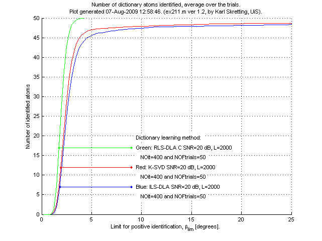
Above is results for ex211.m.
We see that the RLS-DLA method here performs better than ILS-DLA (MOD) and K-SVD which both perform quite similar.
The most remarkable difference is that RLS-DLA is able to identify all atoms for a
quite small angle βlim. ILS-DLA (MOD) and K-SVD always have some
atoms that are far away from the true atom. Having βlim=8.11 degrees
corresponds to the case where the inner product of the two compared atoms is equal to 0.99,
each atom has 2-norm equal to 1.
This section describes how to learn the dictionaries used in the image compression examples in our ICASSP 2011 paper. How the learned dictionaries were used is described in the image compression example in section 7 on the IC tools page where also the 8 used dictionaries are available, those dictionaries were designed by the m-files presented here. An important point in our ICASSP 2011 paper is that sparse approximation using a dictionary can be done in the coefficient domain, and that this improves compression performance in much the same way as using the 9/7 wavelet transform performs better than using the block dased discrete cosine transform (DCT). Thus, the learning must be done in the coefficient domain and the training vectors be in the coefficient domain.
A Matlab function, getXfrom8images.m,
was made to generate the training vectors from 8 training images (shown below).
The function is actually quite flexible and can be used to generate training vectors from
all images that can be read by the Matlab imread function.
Training vectors can be made in the pixel domain or in several transform domains, most important the 9/7 wavelet domain.
The function needs mycol2im.m from ICTools,
which must be in the current directory or available on the Matlab search path.
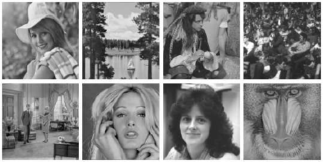
The getXfrom8images.m file should be updated so that its default image catalog matches a catalog
on your computer where the 8 bmp-images above, i.e. elaine.bmp, lake.bmp, man.bmp, crowd.bmp,
couple.bmp, woman1.bmp, woman2.bmp, baboon.bmp, are all stored.
These images, as well as lena.bmp, are available in a zip-file,
USCimages_bmp.zip.
Having access to the set of training vectors we could start learning dictionaries using the
dlfun.m briefly presented in the beginning of section 3 here. But the function is slow.
Here we have made four Matlab functions more appropriated, in the sence that they are more
directed towards the image compression problem at hand and faster than dlfun.m.
The four files are denoted as ex31?.m, where ? can be 1 for ILS-DLA (MOD) learning,
2 for RLS-DLA learning, 3 for K-SVD learning and 5 for a special separable MOD learning.
The three first methods are briefly explained in section 3 above, and the separable case is
described in section 3.6 in my PhD thesis.
The four functions are all used in a very similar way, like:
%    res = ex31?(transform, K, targetPSNR, noIT, testLena, verbose);
%-------------------------------------------------------------------------
% where the arguments are:
%   transform   may be:  'none', 'dct', 'lot', 'elt', 'db79', 'm79'
%               see myim2col.m (in ICTools) for more
%   K           number of vectors in dictionary
%               for the separable case use [K1, K2] instead of K
%   targetPSNR  target Peak Signal to Noise Ratio, should be >= 30
%   noIT        number of iterations through the training set
%   testLena    0 or 1, default 0. (imageapprox.m is used)
%   verbose     0 or 1, default 0.
%-------------------------------------------------------------------------
The returned variable res will be a struct with the leared dictionary as one field.
It will also be stored in a mat-file in the current catalog.
The 8 dictionaries learned for the image compression example in section 7 of the ICTools page
were learned by these four implementations.
The m-file ex31prop.m can be used to display some properties of these dictionaries,
and other dictionaries learned by the four m-files ex31?.m.
For example, the results of r=ex31prop('ex31*.mat', 'useLaTeX',true); is:
ex31prop display properties for 8 dictionary files.
\hline
Dictionary filename   & iter & tPSNR & trans. &     A &     B & betamin & betaavg \\
\hline
 ex311Feb031626.mat   & 1000 &  38.0 & none   &  0.09 & 73.73 &    7.84 &   43.43 \\
 ex311Jan241424.mat   & 1000 &  38.0 & m79    &  0.14 & 57.20 &   12.03 &   46.37 \\
 ex312Jan191930.mat   &  800 &  38.0 & m79    &  0.58 & 30.54 &   16.18 &   54.05 \\
 ex312Jan282133.mat   &  500 &  38.0 & none   &  0.47 & 30.96 &   16.36 &   53.86 \\
 ex313Feb011544.mat   & 1000 &  38.0 & none   &  0.23 & 63.58 &    4.71 &   45.91 \\
 ex313Jan251720.mat   & 1000 &  38.0 & m79    &  0.30 & 54.68 &    9.03 &   48.01 \\
 ex315Feb021040.mat   & 1000 &  38.0 & none   &  0.92 & 27.57 &   19.62 &   35.67 \\
 ex315Jan211232.mat   &  500 &  38.0 & m79    &  0.70 & 20.38 &   30.36 &   41.16 \\
\hline
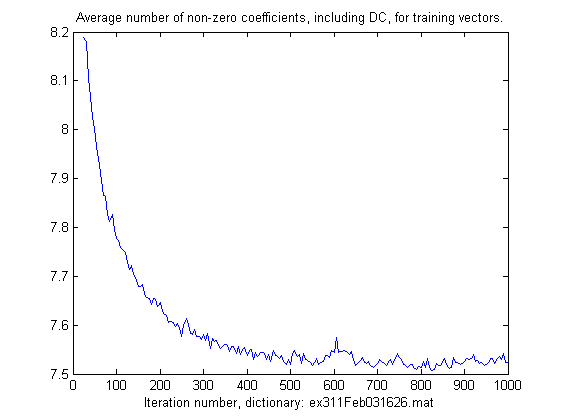
During learning the four m-files ex31?.m saves some information to show the progress of learning.
Since the target PSNR is fixed, some of the first iterations are used to find an appropriate limit for the error
which is used as a stopping criterion in sparse approximation. After some few iterations the achieved
PSNR is quite stable during learning and as the dictionary further improves the average number of non-zero
coefficients for each training vector slowly decreases. This can be plotted, for example:
  r1 = load('ex311Feb031626.mat');
  r1.tabPSNR(1:10)'  % display the first PSNR values (on the next lines)
ans =
   35.8615   38.2784   37.8627   38.0553   37.9764   38.0124   37.9938   37.9985   38.0014   38.0004
   plot(r1.tabIT(5:end), r1.tabNNZ(5:end)/r1.L);
   title('Average number of non-zero coefficients, including DC, for training vectors.');
   xlabel(['Iteration number, dictionary: ',r1.ResultFile]);
The result off the commands above is plotted below.
This section starts with a brief presentation of some dictionary properties. Many of these properties are used in the experiments done in the SPIE paper, they are used to assess learned dictionaries and to compare dictionaries to each other. The larger part of this section describes two of the three experiments done in the SPIE paper. The main purpose of these experiments were to compare different learning algorithms to each other, including the effect of using either the l0-norm (ORMP) or l1-norm (LARS) in vector selction, for sparse approximation of patches from natural images. The Matlab files and how to use them are briefly explained. Some results are presented, including plots of some of the learned dictionaries.
A thorough presentation of many dictionary properties is given in
Elad's book: "Sparse and Redundant Representations ...".
Also the SPIE 2011 paper gives an overview of some dictionary properties, mainly those that are relatively easy to compute.
It also suggests some new properties, i.e. μmse, μavg,
βmse, and βavg, and proposes a measure for the
distance between two dictionaries: β(D,D').
The table below lists some properties for a normalized dictionary, i.e. each atom (column vector) has unit 2-norm.
The dictionary is represented as a matrix D of size NxK.
For more details on each property see the SPIE paper.
| Property | Definition (comment) |
|---|---|
| σ1, σ2, ... σN | The singular values of D, where we assume
σ1 ≥ σ2 ≥ ... σN |
| λ1, λ2, ... λN | The eigenvalues of the frame operator S=DDT,
we have λi = σi2
and Σi λi = K |
| A, B | Lower and upper frame bound, A = λN and B = λ1 |
| μ, βmin | Coherence and angle between the two dictionary atoms closest to each other, coherence is cosine of the angle. For a normalized dictionary the coherence is the inner product of the two closest atoms. |
| μavg, βavg | Average of cosine (angle) for all atoms to its closest neighbor. |
| μmse, βmse | Average, in mean square error sense, of cosine (angle) for all pairs of atoms in the dictionary, including an atom to itself. These properties can be computed from the eigenvalues. |
| μgap, βgap | Cosine (angle) for the most difficult vector x to represent by one atom
and its closest neighbor in the dictionary. This property is generally hard to compute. |
δ(D) |
The decay factor used in Elad's book,
we have δ(D) = μgap2 |
β(D,D') |
Distance between two dictionaries as the average angle between each atom (in both dictionaries) to its closest atom in the other dictionary. |
SRC |
The Sparse Representation Capability is the average number of atoms used in a sparse approximation of a set of test vectors where the representation error is below a given limit for each test vector. |
We will here present the two first of the three experiments presented in the SPIE paper. A general description of the experiments and the main result are given in the paper. This web-page mainly presents the Matlab files needed to redo the experiments, but also some results not given in the paper are shown. In all experiments training vectors are generated from 8 by 8 patches from natural images in the Berkeley image segmentation set. The files were copied into a catalog on the local computer, and a Matlab function, getXfromBSDS300.m, was made to access the data in an easy way. Note that you have to change some few lines in this m-file (near line 175) to match the catalog where you have copied the data on your local computer. Matlab example:
  par = struct('imCat','train', 'no',1000, 'col',false, 'subtractMean',true, 'norm1lim',10);
  X = getXfromBSDS300(par, 'v',1);
The following table shows some example dictionaries.
| Dictionary, size is 64x256 | Atoms | mat-file | A | B | μmse | μavg | μ | SRC |
|---|---|---|---|---|---|---|---|---|
| 1. Random Gaussian |
|
dict_rand.mat |
1.12 | 9.10 | 0.1405 | 0.3709 | 0.5803 | 14.86 |
| 2. Patches from training images |
|
dict_data.mat |
0.07 | 49.87 | 0.2860 | 0.6768 | 0.9629 | 11.20 |
| 3. RLS-DLA learned dictionary (from ex.1) |
|
ex414_Jun250624.mat |
0.13 | 17.89 | 0.1596 | 0.5205 | 0.9401 | 8.37 |
| 4. Orthogonal bases |
|
dict_orth.mat |
4 | 4 | 0.1250 | 0.1250 | 0.1250 | 10.87 |
| 5. Separable dictionary with sine elements |
|
dict_sine.mat |
1.00 | 6.66 | 0.1350 | 0.4971 | 0.4999 | 9.89 |
| 6. Dictionary with sine elements and corners |
|
dict_ahoc.mat |
1.47 | 6.15 | 0.1318 | 0.5026 | 0.6252 | 9.14 |
The dictionaries listed in the table are available as mat-files, links are given in third column. Some dictionary atoms are shown in the second column of the table, all atoms should be shown when you click on these. The six rightmost columns are properties found for each dictionary. The fourth dictionary is the concatenation of 4 maximally separated orthogonal bases, it is made by the get64x256.m function. The dictionary in the table includes the identity basis, and the SRC measure is 10.87. If we rotate all atoms such that the 2D-DCT basis is in the dictionary (instead of the identity basis) then we get a dictionary with the same properties but which will achieve better SRC measure, SRC = 10.38. Using only the dct basis will give SRC = 13.55. The fifth dictionary is made by the get64x256sine.m function which needs the getNxKsine.m function. The last dictionary is an ad-hoc dictionary with 168 separable sine atoms, and the rest of the atoms are 6x6 2D-dct basis functions multiplied by a window-function and located in the corner of each patch.
For the dictionaries in experiment 1 and 2 it was convenient to make a special function to
find and return the dictionary properties, mainly because the special SRC measure is also wanted.
To find SRC a specific set of test data should be available and stored in a mat-file in current directory,
the file used here is testDLdataA.mat (7.5 MB) and contains 25600 test vectors
generated from the Berkeley image segmentation test set. The function should also plot the development of
some of the properties during learning, when available these are plotted in figure 1 to 3,
and display the dictionary atoms in yet another figure, here figure 4.
The result is a 'quick-and-dirty' m-file, testDLplot.m.
This function needs a struct containing the dictionary and possible also learning history as fields,
alternatively the name of a mat-file containing this struct with the name res, as the first input argument.
For most dictionaries the more clean and tidy functions dictprop.m
and dictshow.m should be used.
Anyway, you may try the following code:
  v = testDLplot('ex414_Jun250624.mat', 1);
  % or
  clear all;
  load dict_rand.mat    % or dict_data.mat, dict_orth.mat
  res.D = D;            % since D is stored, but a struct is needed in testDLplot
  v = testDLplot(res, 1);
  % or
  clear all;
  res.D = get64x256('dct');  % a 'better' alternative to the fourth dictionary
  v = testDLplot(res, 1);
In experiment 1 the RLS-DLA algorithm was used and different parameters were used, see SPIE paper. To make similar dictionaries you may try the code in ex414.m, note that this is not a function but simply a collection of Matlab commands. ex414.m uses the java-function DictionaryLearning.rlsdla(..) which unfortunately only uses the sparse approximation methods implemented in the same package. Thus to use RLS-DLA with LARS, i.e. mexLasso in SPAMS, the function denoted testDL_RLS.m is needed. Both these m-files store the dictionary as a struct in a mat-file. Examples of use are:
  clear all; ex414;    % all defaults
  % or
  clear all;
  dataSet='A'; batches=100; dataLength=20000; lambda0=0.996; targetPSNR=38;
  ex414;
  v = testDLplot(res, 1);
  % or
  param = struct('vecSel','mexLasso', ...
                 'mainIt',100, ...
                 'dataLength',20000, ...
                 'dataSet','A', ...
                 'dataBatch',[20*ones(1,20),50*ones(1,50),100], ...
                 'targetPSNR', 38, ...
                 'lambda0', 0.998  );
  res = testDL_RLS( param );
  v = testDLplot( res, 1 );
Varying targetPSNR and lambda0 it should be possible to make dictionaries similar to the ones described in the SPIE paper, and present the results in a similar way. We observed that the resulting dictionary properties mainly depended on the selected parameters. Learning several dictionaries with the same parameters, but different initial dictionary and different training vectors, all had almost the same properties. This is a good property of the learning algorithm, as it seems to capture the statistical properties of the training set rather than depending on the specific data used. We also noted an essential difference between dictionaries learned by LARS (l1-sparsity) and dictionaries learned by ORMP (l0-sparsity), see results presented in the SPIE paper.
In experiment 2 we again refer to the SPIE paper for a more complete description of the experiment and a presenteation of the results. This section presents the Matlab files and some additional results. First we review the main results as presented in Table 3 in the SPIE paper.
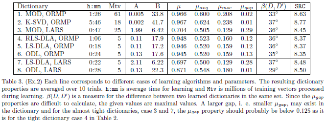
The 8 different (variants of) dictionary learning algorithms used in this experiments are implemented by 4 m-files. The MOD dictionaries, case 1 and 3, were generated by testDL_MOD.m. The K-SVD dictionaries, case 2, were generated by testDL_KSVD.m. These two functions assume that there is available a fixed huge set (1 million vectors) of training vectors in 50 files (20000 training vectors in each) in a catalog on the local computer. But if these files are not available the functions will make a new set of training data in each iteration. The advantage with a fixed, but huge, training set is that learning has a fixed training set, which is an assumption made when the algorithms are derived. But even with this huge training set, in each iteration only some few (1 to 10 randomly chosen) subsets of the 50 available subsets are used, and this way the 'fixed training set in each iteration' assumption is violated. The dictionaries for the first three cases can be made by the Matlab commands below, the results can be displayed by testDLplot.m function.
  p1 = struct('vecSel','mexOMP', 'targetPSNR',38, 'mainIt',1000);
  p2 = struct('vecSel','mexOMP', 'targetPSNR',38, 'mainIt',500);
  p3 = struct('vecSel','mexLasso', 'targetPSNR',35, 'mainIt',400);
  % more parameters can be used to do logging in each iteration during learning
  pExtra = struct('useTestData',true, 'verbose', 1, ...
                  'avg_w0',1, 'avg_w1',1, 'avg_r2',1, 'avg_rr',1 );
  res1 = testDL_MOD(p1);   % or  res1 = testDL_MOD(p1,pExtra);
  res2 = testDL_KSVD(p2);  % or  res2 = testDL_KSVD(p2,pExtra);
  res3 = testDL_MOD(p3);   % or  res3 = testDL_MOD(p3,pExtra);
The dictionaries in case 4 were made by the ex414.m m-file used in experiment 1, but with different parameters. The last 4 cases were all made by the ex413.m m-file, this is a function and may be called with several parameters to select which variant of ODL or LS-DLA to run. The two different methods were implemented by the same function since the implementation should ensure that the two methods, ODL and LS-DLA, can be run under exactly the same conditions. It should be possible for both methods to use excactly the same scheme for the forgetting factor and for the mini-batch approach, the only difference is the few code lines where the actual dictionary update is done. ODL uses the equation 3.4 in section 3.3 above, while LS-DLA uses the equation 3.3 in section 3.1 above. The LS-DLA scheme is actually how we would implement a mini-batch variant of RLS-DLA. We see that the true RLS-DLA implementation in case 4 and the mini-batch implementation in case 5 give dictionaries with the same properties. The dictionaries for the last five cases can be made by the Matlab commands below, the results can be displayed by testDLplot.m function.
  clear all;
  batches=250; dataLength=20000; lambda0=0.996; targetPSNR=40;
  ex414;
  res4 = res;
  % total number of vectors processed is: sum(mb(:,1).*mb(:,2))
  mb = [2000,50; 5000,100; 10000,200; 5000,250; 2300,500];
  p5 = struct('vecSel','mexOMP', 'lambda0',0.996, 'targetPSNR',40, ...
              'ODLvariant',5, 'minibatch',mb);
  res5 = ex413(p5);
  p6 = p5; p6.ODLvariant = 2;
  res6 = ex413(p6);
  p7 = struct('vecSel','mexLasso', 'lambda0',0.998, 'targetPSNR',35, ...
              'ODLvariant',5, 'minibatch',mb);
  res7 = ex413(p7);
  p8 = p7; p8.ODLvariant = 2;
  res8 = ex413(p8);
The distance between two dictionaries, β(D,D') in Table 3 in SPIE paper,
shows that dictionaries learned by the same method are in fact quite different from another,
even though their properties are almost the same.
The variance (or standard deviation) is relatively small for all values in Table 3, also for
the β(D,D') measure. That means that if two dictionaries are learnt by the
same method, and the same parameter set, the expected distance between them will be expected to
be as given in Table 3, standard deviation will be less than 1 degree.
We can also measure the distance between dictionaries from different cases and present the
results in a table, the column in Table 3 in the SPIE paper is the diagonal in this table.
| Case | 1 | 2 | 3 | 4 | 5 | 6 | 7 | 8 |
|---|---|---|---|---|---|---|---|---|
| 1 | 33.40 | 35.86 | 39.90 | 35.62 | 35.67 | 35.38 | 40.29 | 36.68 |
| 2 | . | 37.07 | 42.49 | 38.45 | 38.49 | 38.29 | 42.93 | 38.87 |
| 3 | . | . | 35.90 | 40.24 | 40.29 | 40.04 | 36.80 | 42.58 |
| 4 | . | . | . | 35.57 | 35.60 | 35.36 | 40.39 | 39.39 |
| 5 | . | . | . | . | 35.75 | 35.44 | 40.47 | 39.56 |
| 6 | . | . | . | . | . | 34.81 | 40.20 | 39.11 |
| 7 | . | . | . | . | . | . | 36.85 | 43.17 |
| 8 | . | . | . | . | . | . | . | 28.57 |
We note that the thre cases 4, 5 and 6 are almost equal to each other, especially 4 and 5.
Also case 3 and case 7 are quite equal to each other, these numbers are shown bold in the table.
This table also hows that dictionaries for case 8 are quite special, they are different from the other cases
and also more clustered, i.e. more equal to each other in the β(D,D') measure.
For experiment 3 we just refer to the SPIE paper.
The experiments are done in Matlab supported by Java.
The Java package mpv2
is a collection of all the Java classes used here.
mpv2 stands for Matrix Package version 2 (or Matching Pursuit version 2).
Note that mpv2 is compiled for Java 1.5 and does not work with older Java Virtual Machines (JVM),
upgrading JVM in Matlab is possible, see
Mathworks support.
mpv2 has classes for Matching Pursuit based vector selection algorithms and for Dictionary Learning Algorithms.
The ILS-DLA (MOD) and RLS-DLA methods are implemented in this package.
As the classes for MP and DLA use matrices extensively, effective Java
implementations of some matrix operations were also needed. This was done by
including the classes from the JAMA-matrix package
and wrapping an abstract matrix class
AllMatrices
around the implementations of different kind of matrices, including the JAMA-matrix class.
The mpv2 package works well,
and I think that parts of the package are well designed and easy to use.
But the mpv2 package must still be regarded to be incomplete and under development.
To use the mpv2 Java package from Matlab you need to copy the class-files
from mpv2-class.zip
into a catalog available from a Java Path in Matlab.
For example you may copy the unzipped class-files into the catalog F:/matlab/javaclasses/mpv2/,
and make the catalog F:/matlab/javaclasses/ available in Matlab as a
DYNAMIC JAVA PATH (see Matlab javaclasspath).
Documentation is in mpv2.
Java files, i.e. source code, for most classes in the mpv2 package are in
mpv2-java.zip.
I consider the left out classes, DictionaryLearning and MatchingPursuit,
to be of less general interest.
If you want to run these experiments you should make a catalog in Matlab where you put all Matlab-files
from the table below. To test that the files are properly installed you start Matlab and go to
the catalog where the files are installed. In the Matlab command window type
help lambdafun to display some simple help text, then go on and type
lambdafun('col'); to run the function and make a plot.
The file java_access check that the access to the mpv2 Java package is ok.
You should probably edit this m-file to match the catalog where mpv2 is installed.
When Java access is ok you may run bestAR1. This file uses the ORMP algorithm (javaORMP)
to do a sparse representation of the AR(1) training set using a predesigned dictionary.
| mat-files | Text |
|---|---|
| bestDforAR1.mat | The mat-file which store the best dictionary for the AR(1) data. |
| dataXforAR1.mat | The mat-file which store the training, and test, data set. Size is 16x4000. |
| dict_ahoc.mat, dict_data.mat dict_orth.mat, dict_rand.mat dict_sine.mat |
5 example dictionaries used in section 5.2 above. |
| ex414_Jun250624.mat | An example dictionary made by ex414.m, see section 5.2 above. |
| testDLdataA.mat | The mat-file with data used for the SRC-measure in section 5.2 above. Size is 64x25600. |
| m-files | Text |
| bestAR1.m | Load and test the best (found so far and using ORMP with s=4) dictionary for the special set of AR(1) data, i.e. bestDforAR1.mat. |
| datamake.m | Generate a random data set using a given dictionary. |
| dictdiff.m | Return a measure for the distance between two dictionaries. |
| dictlearn_mb.m | Learn a dictionary by a minibatch RLS-DLA variant. |
| dictmake.m | Make a random dictionary, iid Gaussian or uniform entries. |
| dictnormalize.m | Normalize and arrange the vectors of a dictionary (frame). |
| dictprop.m | Return properties for a normalized dictionary (frame). |
| dictshow.m | Show atoms, basis images, for a dictionary or a transform. Needs mycol2im.m from ICTools. |
| dlfun.m | A slow Matlab only Dictionary Learning function, can be used for MOD, K-SVD, ODL or RLS. |
| ex111.m, ex112.m | m-files for first experiment presented in section 4.1 here. |
| ex121.m | m-file for second experiment presented in section 4.1 here. |
| ex131.m, ex132.m | m-files for third experiment presented in section 4.1 here. |
| ex210.m, ex211.m | m-files for generating data and displaying results for experiment presented in section 4.2 here. ex210.m is extended with more learning alternatives April 2013. |
| ex300.m | m-file that tests sparseapprox.m, using the mat-files above. |
| ex311.m, ex312.m ex313.m, ex315.m |
Dictionary learning for images, section 5.1 above. The metods are ILS-DLA (MOD), RLS-DLA, K-SVD and separable MOD. |
| ex31prop.m | Display some properties for dictionaries stored in ex31*.mat files. |
| ex413.m, ex414.m | Dictionary learning for (BSDS) images, section 5.2 above. |
| getNxK.m | Get a NxK dictionary (frame) with small coherence, use L-BFGS. |
| getNxKsine.m | Get a NxK dictionary (frame) with or without sine elements. For the case without sine elements a small coherence dictionary is returned. |
| get8x21haar.m | Get an 8x21 regular Haar dictionary (frame), used in ex315.m. |
| get8x21sine.m | Get an 8x21 dictionary (frame) with sine elements, used in ex315.m. |
| get16x144.m | Get a 16x144 tight dictionary (frame). |
| get64x256.m, get64xK.m | Get a 64x256, or a 64xK, tight dictionary (frame). |
| get64x256sine.m | Get a 64x256, i.e. (8x8)x(16x16), separable dictionary with sine elements. |
| getXfrom8images.m | Get (training) vectors generated from 8 example images. |
| getXfromBSDS300.m | Get (training) vectors generated from images copied from the Berkeley image segmentation set. |
| lambdafun.m | Can be used to set the forgetting factor λ in RLS-DLA. |
| idxSIDmap.m | Index map between SID dictionaries of different size. |
| initSID.m | Initialize Shift Invariant Dictionary given atom lengths and shifts. |
| initSID2D.m | Initialize Shift Invariant Dictionary for the two dimensional case |
| makeSIDmatrix.m makeSID2Dmatrix.m |
Make sparse matrix D from Shift Invariant Dictionary, 1D case and 2D case |
| multSID.m, multSIDt.m multSID2D.m |
Multiplication for Shift Invariant Dictionary (SID): y = D*w and c = D'*y and the two dimensional case y = D*w. |
| plotSID.m | Visualize Shift Invariant Dictionary. |
| plotSID2D.m | Visualize Shift Invariant Dictionary for the two dimensional case |
| saSIDbmp2.m | Sparse Approximation using Shift Invariant Dictionary (SID) and Matching Pursuit (MP). |
| saSIDomp.m, saSID2Domp.m | 1D and 2D variants of Orthogonal MP using Shift Invariant Dictionary. |
| testDL_MOD.m, testDL_RLS.m testDL_KSVD.m, testplot.m |
Dictionary learning for (BSDS) images, section 5.2 above, and a special varint for plotting (showing) dictionary properties. |
| more files | Text |
| assignmentoptimal.m | Compute optimal assignment by Munkres algorithm (by Markus Buehren). |
| java_access.m | Check, and try to establish, access to mpv2 java-package. Some statements in this file should be changed to reflect the catalog structure on your computer, and perhaps also use a m-file like below to return the relevant path. |
| munkres.m | Compute optimal assignment by Munkres algorithm (by Yi Cao), faster than assignmentoptimal.m. |
| my_matlab_path.m | Return the relevant path for (some of) my matlab catalogs. |
| saSIDbmp_mex.c saSIDbmp_mex.mexw64 |
Sparse approximation using Shift Invariant Dictionary (SID) and method Basic Matching Pursuit. and compiled for Matlab in Windows 64 bit. |
| sparseapprox.m | Returns coefficients in a sparse approximation of each column in a matrix X. |
| sparse_xcorr_mex.c sparse_xcorr_mex.mexw64 |
Sparse xcorr variant implemented directly in time domain (not via FFT). and compiled for Matlab in Windows 64 bit. |
| zip-files | Text |
mpv2-class.zip |
The class-files for the mpv2 Java package. |
mpv2-java.zip |
The java-files for most of the classes in the mpv2 Java package. |
USCimages_bmp.zip |
Some images stored as bmp files, once copied from the
University of Southern California-SIPI image database. The directory where these are stored should be written into the getXfrom8images.m file. |
The MATLAB files are quite old but should still function as they did 10–15 years ago. However, since then, Python has gained significant popularity as a programming language, and many users—students, researchers, or others—may prefer to use Python instead. To accommodate this, several of the main algorithms described above have now (as of 2025) been implemented and are available as Python functions.
Some of these algorithms are included in Python libraries such as scikit-learn, but others—like Partial Search, RLS-DLA, and mini-batch dictionary learning—are, to my knowledge, not available in any standard Python packages.
Many of the provided Python functions use Numba to accelerate execution. However, they should still work (albeit more slowly) even if Numba is not installed. For example, the 2D 9/7 wavelet transform (3 levels), implemented using the lifting scheme and Numba, achieves performance comparable to the 2D DCT from scipy.fft. See the lwt97 and ilwt97 functions in funImageTransform.py for details.
The complete Python codebase is organized into multiple files, typically in pairs: one file containing the core functions (fun*.py) and a corresponding test file (test*.py) that uses unittest to demonstrate and verify functionality. The code relies on standard Python packages such as sys, numpy, and others, and often imports functions from other fun*.py modules.
| py-files | Text |
|---|---|
| funSparseApprox.py testSparseApprox.py |
Functions for sparse approximation (OMP/ORMP and Partial Search) and a program (unittest) to test these funtions. |
| py_fun_and_test.zip | 11 pairs of fun*.py and test*.py files |
| Last update: July 3rd, 2025. Karl Skretting | Visit my home page. |