Karl Skretting, University of Stavanger.
| Contents on this page: | Relevant papers and links to other pages: |
|---|---|
|
Many different image compression schemes exist, and several, often completely, different methods can be used for each of the different steps in an image compression scheme, and the different methods can often be combined in any way. Some examples are the Matlab implementation of SPIHT which is used as a reference compression scheme here. Also Matlab commands imwrite and imread supports several image formats, many of them include effective compression. The latest versions (from R2010b) also support the effective JPEG-2000 format (JP2 option). The standard JPEG format is also supported but the compression rate is not as good as expected, perhaps the overhead information is relatively large.
This page contains several Matlab functions, m-files, a brief explanation and some examples for image compression. The included functions can be used for some of the many steps or stages often done in image compression. It is not a complete finished codec, like JPEG or JPEG-2000. The stages presented here, section 2 to 6, are, with some variants, used in most image compression schemes. The more special method presented in section 7 can be used instead of, or in addition to, the transform part, section 3. Also several of these steps may be used for compression of other signals, or for other tasks in signal processing.
The task of preprocessing is to present the image to the next stages in an appropriate format. This includes reading the image file, and possible separate different layers of the image, divide the image into tiles, adjust size, subtract mean and scale the image. In Matlab a bitmap-file, ex. lena.bmp, can be read (into doubles) by
A = double(imread('lena.bmp'))-128;
If the image A is in the
RGB color space
the different colors are in A(:,:,1),
A(:,:,2) and A(:,:,3).
In Matlab the RGB color space can be transformed into
YCbCr color space by
    [M,N,Layers] = size(A);   % RGB: Layers==3
    T = [   0.299,    0.587,    0.114; ...
           -0.16875, -0.33126,  0.5; ...
            0.5,     -0.41869, -0.08131  ];
    A(:,:,1:3) = permute(reshape(T*reshape(permute(A(:,:,1:3),...
                    [3,1,2]),3,M*N),3,M,N),[2,3,1]);
    A = A(:,:,1);  % first (luminance) layer only
Further processing is done on each layer independently of other layers.
It is often necessary that the image size,
M and N in the example above,
is a factor of a number given by the transform size, typically 8, 16 or 32.
To adjust the image size different methods can be used,
this can be done by myimadjust.m.
For example to add rows of zeros at the bottom, or columns of zeros to the right,
such that both height M and width N have 16 as a factor use
    A = myimadjust(A, 'zeros', 16);
    [M,N] = size(A);   % adjusted size
The image can be transformed into a coefficient domain in many ways. Common methods are block transforms, usually separable ones, like the Discrete Cosine Transform (DCT) used in JPEG. Alternatives are overlapping transforms, like Lapped Orthogonal Transform (LOT) and Extended Lapped Transform (ELT). Wavelet based transforms perform very well on images, popular wavelet transforms are the bi-orthogonal 9/7 and the 5/3 wavelet filters which are both used in the JPEG-2000 compression scheme. Wavelets can be implemented by the effective Lifting scheme. Also, both wavelets and lapped transforms are special cases of filter banks and they can be implemented the same way as an overlapping transform. For images this is done in a separable way, independently applying the transform both by rows and by columns.
After the transform the image is represented by the transform coefficients,
usually the number of coefficients is equal to the number of elements (pixels) in the image.
These may be organized in many ways, the different sub-bands may be separated
or they may be interlaced, they may be organized as blocks (transforms) or as trees (wavelets).
A common method is to do the transform in-place, and then the coefficients
are stored in a M-by-N matrix like the image.
This matrix can be divided into blocks, which size is given by the size of the transform,
such that the coefficient in one position of one block belongs to the same sub-band
as a coefficient in the same position in any other block.
Let the block have size Ms-by-Ns, then each block can be ordered into a column vector,
which can be collected into a matrix X of size (Ms·Ns)-by-L
where L=(M·N)/(Ms·Ns) is number of blocks.
All elements of one row (of matrix X) belong to the same sub-band,
but for some transforms, i.e. wavelets, one sub-band may occupy several rows.
I have made a flexible function, myim2col.m, which may both do a transform
and organize the coefficients as a matrix X.
The inverse function, mycol2im.m, go the opposite way,
a coefficient matrix X is reshaped and transformed into an image A.
Below is examples that do the common 8-by-8 2D DCT and the LOT transform.
myim2col.m uses getLOT.m to get the LOT overlapping
synthesis vectors, a matrix of size 16-by-8 organize coefficients into 8-by-8 blocks.
    X = myim2col(A, 't','dct', 's',8);   %  8x8 DCT
    X = myim2col(A, 't','lot', 's',8);   % 16x8 LOT
To do the lifting scheme for wavelets myim2col.m uses my own
lifting implementation, mylwt2.m.
This works essentially like the Matlab Wavelet Toolbox function lwt2.m,
except that mylwt2.m does mirroring at the image edges
while lwt2.m does zero-padding.
Two variants of the popular 9/7 wavelet is available in mycol2im.m,
the 'm97' value (mirror 9/7) for option 't' (transform) scale
low-pass band and high-pass band of the wavelet such that it is close to
orthogonal, i.e. the energy distribution between low-pass band (or DC) and high-pass band is kept,
the alternative 'j97' value is like in JPEG-2000 and amplifies low-pass band more
than high-pass band which often gives better visual result in compression.
A wavelet can also be implemented using a matrix representing the wavelet as
an overlapping transform, to get this matrix I made the function GetWave.m.
Note that in this case a separable transform is done, independently dividing
each direction into (level+1) sub-bands, a total of 16 sub-bands for a 3 level wavelet.
Lifting only process the low-low-band in the next level giving a total of
(3·level+1) sub-bands, for 3 levels this is 10 sub-bands.
Also note that the implementation of overlapping transform in mycol2im.m
do periodic extension of the columns and the rows.
Examples of how to use mycol2im.m are below, note that the
three different results, X matrices, will not be equal to each other.
See help text for mycol2im.m to get an overview of all options,
and see test01.m for many more examples of use.
    X = myim2col(A, 't','m97', 's',8);   %  9/7 wavelet (lifting) 3 levels
    % using Matlab Wavelet Toolbox (zero padding)
    LS = {'d', -1.586134342059924*[1,1], 1; ...
          'p', -0.052980118572961*[1,1], 0; ...
          'd',  0.882911075530934*[1,1], 1; ...
          'p',  0.443506852043971*[1,1], 0; ...
          1.230174104914001, 1/1.230174104914001, []};  % as in JPEG-2000
      %   1.1496, 1/1.1496, []};  % more equal distribution of energy
    Y = lwt2(A, LS, 3);
    X = im2col(Y, [8,8], 'distinct');
    % and wavelet as an overlapping transform
    G = GetWave('db79a',3);   % 3 levels of 9/7 wavelet ==> G is a 64x8 matrix
    X = myim2col(A, 't',G, 's',[8,8]);
In its basic form quantization is simply rounding the real values of the coefficients into nearest integers. More generally scalar quantization is a mapping from a continuous interval into integers, i.e. dividing the interval into non-overlapping bins and assigning an integer to each bin. Quantization removes information (accuracy) from the numbers and thus introduces error during reconstruction; the reconstructed value is usually the bin center. Often more advanced ways of quantization are used. JPEG scales each sub-band by a factor before rounding to integers, the factors are chosen considering the human visual system which is more sensitive to low-frequency noise than high frequency noise. JPEG-2000 may vary the quantization step size for each sub-band, and use a larger zero-bin. Also, truncation during bit-plane coding may be considered as a form of quantization.
The examples here use a simple uniform quantization with thresholding, i.e. all bins are equal size except zero-bin which may be larger. Usually, the zero-bin is twice the size of other bins. The implementation is in uniquant.m.
The reconstruction error can be measured by the Peak Signal to Noise Ratio, PSNR.
Having the original image A including the peak, for 8 bit pixel values this is 255,
and the reconstructed image Ar PSNR can be found as
    peak = 255;
    X = myim2col(A, 't','m97', 's',8);   %  9/7 wavelet (lifting) 3 levels
    del = 10;
    thr = del;  % zero bin from -thr to thr, here twice the size of other bins
    Z = uniquant(X, del, thr, 2000);  % Z will not be larger than 2000 (truncation value)
    Xr = uniquant(Z, del, thr);  % inverse quantizing
    Ar = mycol2im(Xr, 't','m97', 's',8, 'imsize',size(A));
    R = A-Ar;    % reconstruction error
    PSNR = 10*log10(((numel(A)*peak^2)/sum(sum(R.*R))));
The matrix Z after scalar quantization is of same size as
the matrix X after transform, and its elements are integers.
This matrix should be coded without loss.
If the transform is appropriate for the image the Z matrix will have a structure,
many elements will be zeros, and these zeros will often be clustered.
A good coding strategy takes advantage of this in an effective way.
Here, the coding is done in two steps. First reshaping the Z matrix
into sequences of integers, and then these sequences are entropy coded.
A large number of techniques are available when building these sequences.
First row of the Z matrix should contain the DC component of the image
after the transform. This is the most important sub-band for natural images,
and represents by itself a crude representation of the image.
Since neighboring pixels in an image often have almost the same values,
difference coding (DPCM) of this row may be helpful, i.e. instead of each value
the difference from the previous value is stored. This coding can be reversed without loss.
Two small functions can do this:
    function y = thisDPCM(x)
    x = x(:);
    y  = [x(1); x(2:end)-x(1:(end-1))];  % [x(1); diff(x(:))] is the same
    return;

    function x = invThisDPCM(y)
    x = zeros(numel(y),1);
    x(1) = y(1);
    for i=2:numel(y);
        x(i) = x(i-1) + y(i);
    end
    return
Since the DC sub-band, first row of Z, represents a crude representation of the image it has
a two-dimensional structure like an image. Prediction of each new element pixel can then
be made more complex, and better, than simple DPCM by exploiting the two dimensional structure.
It is also possible, and helpful, to predict not only the value of next element but
also the magnitude, or variance, of the prediction error. The prediction errors with
small estimated variance can be put in one sequence and the prediction errors
with larger estimated variance in another sequence. The resulting sequences will probably
have different distribution of the symbols (integers) and different
entropy,
and fewer bits are needed to code the two, or more, sequences of prediction errors
than what is needed to code one sequence with all the prediction errors.
I have made a Matlab function that uses this principle, mypred.m.
The prediction scheme can be extended and used on the image itself; this can give quite effective lossless image coding schemes. One of the best schemes based on the prediction model is CALIC (Context-Based, Adaptive, Lossless Image Coder). CALIC is quite complicated, with four major components: 1) Linear prediction, 2) Context selection by estimating the error energy level, 3) Modeling of the prediction error and adjusting it by subtracting a bias, making the final prediction non-linear. 4) Entropy coding of the prediction errors. I have made a Matlab function that is like the first two parts of CALIC, and that return 8 (one for each context) integer sequences, calic.m.
The non-DC sub-bands, all rows of Z except first, may be coded individually
or block-wise. The structure of Z is often so that column-wise
coding of the AC components is best, since each column represent a localized image block.
To do this effectively the rows of Z
should be ordered by ascending frequency, this order is given by the transformation.
An alternative, which works quite well if there is not too many rows is to sort the rows
by the number of non-zeros in each row. Then this order must be included as
an additional integer sequence.
End-Of-Block (EOB) coding uses an extra symbol, EOB, to indicate that the rest of the elements in the column are zero. Arranging the elements from the matrix into one sequence column-wise gives a sequence with the same number of elements, but using an EOB symbol may significantly reduces the number of elements since the zeros often will be at the end of each column. The resulting sequence can further be divided into three sequences depending on the previous symbol, zero, EOB or other. This often improves coding results because after a zero there will never be an EOB symbol, and after an EOB-symbol there will only be symbols from the first row (second row if DC is handled otherwise) or possible EOB symbols.
Run-Length-Encoding (RLE) can be used to better code sequences with many zeros (or another frequent value), especially if this value tends to be clustered. This is often the case with the EOB-sequence of symbols following a zero. One way to do this is to introduce a new symbol, Run-Of-Zeros, which mean two or more zeros. Alternatively it could mean one or more zeros. This symbol is then inserted in the sequence everywhere a run of zeros is present, and the run of zeros is removed. The number of zeros in each run of zeros must be stored in a new sequence. The first sequence may further be divided into two sequences depending on the previous symbol, since we know that after a zero or a Run-Of-Zeros symbol there will always be a non-zero value.
A third method that is efficient if there are many zeros is to make two sequences from the sparse matrix, one sequence with the non-zero values and one with the indexes (DPCM coded). Combining these methods in an effective way may reshape the matrix into sequences that are easier to effectively compress, three variants are implemented in myreshape.m.
Many years ago I implemented Huffman coding and some simple arithmetic coding schemes in Matlab. These functions still works ok, see my Entropy Coding page. They just make the sequences of integers into a sequence of bytes (the bit stream), no packing is done to group the bit stream into independent parts as is an important feature of many image compression schemes. I have also made a function that, if Huff06.m is not available, can estimate the number of bits needed to encode integer sequences based on zero-order entropy of the sequences, estimateBits.m.
Dictionaries can be used to make a sparse representation of the image in the compression scheme, in a similar way that the DCT or wavelet coefficients are often sparse after quantizitation. In our ICASSP 2011 paper it was shown that it is better to do the sparse representation with learnt dictionaries in the wavelet domain than directly in the pixel domain. The compression scheme may be divided into four steps.
Note that the dictionary is not included in the compressed file, as it is supposed to be a general dictionary and an internal part of the compression scheme. Some learnt dictionaries are included in the mat-files numbered 1 to 8 in the table in section 9.2. Atoms or basis images for a dictionary and dictionary properties can be viewed by the Matlab m-files dictshow.m and dictprop.m on the dictionary learning page.
   dict = load('ex312Jan191930.mat');
   A = dictshow(dict);                        % show all 440 atoms
   A = dictshow(dict, 'useK',[1:20,100:135]); % or some given atoms
   p = dictprop(dict.D);
The advantage of step 2 above, compared with DCT or wavelet decomposition with the same error (PSNR), is that the representation is sparser. On the other hand, a disadvantage is that the weight matrix W (including the zeros) is larger, and that the structure in the DCT or wavelet coefficients is lost or hidden, i.e. the non-zero positions in W have a more complex structure, if any structure at all. JPEG, SPIHT and JPEG-2000 exploit the structure in the quantized (DCT or wavelet) coefficients in their advanced entropy coding schemes; especially the EBCOT scheme in JPEG-2000 is advanced and effective.
To do the complete compression of an image using a dictionary is quite complicated. Here it is done using only a single function, imageapprox.m, but it is quite large and perhaps also complicated and several other functions, both on this page and on the dictionary learning page, may be called, for example sparseapprox.m which itself may call many other (complicated) functions. imageapprox.m only use the javaORMP option in sparseapprox.m. The imageapprox function can be controlled by many options, not all possible combinations are tested yet, but with careful use it works quite well. To compress lena with PSNR 38.57 and a bit rate of 0.5 the commands below do the job. Some results are presented in section 8.
   A = double(imread('lena.bmp')) - 128;
   par = struct('dictionary','ex312Jan191930.mat', ...
                'targetPSNR',39.092, ...
                'del',-18, ...   % for adapting (using -del as first)
                'qLimit',[0.38,0.40], ...
                'estimateBits','Huff06', ...
                'verbose',1 );
   res = imageapprox(A, par);
   % store byte sequence and some overhead information
   stored = struct('tr',res.tr, ...        % transform, may be found from dictionary
                   'sizes',res.sizes, ...  % image and transform sizes
                   'del',res.del, ...      % quantizing step, 'thr','deldc','thrdc' may also be given
                   'y',res.y, ...          % the byte sequence (compressed file)
                   'Ds',res.Ds, ...        % the dictionary
                   'ecm',res.ecm   );      % method for entropy coding
   Ar = imagerestore(stored);
   peak = 255;
   R = A - Ar;
   PSNR = 10*log10(((numel(A)*peak^2)/sum(sum(R.*R))));
   disp(['Bit rate is ',num2str(8*numel(res.y)/numel(A)),' and PSNR is ',num2str(PSNR)]);
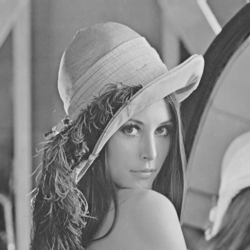
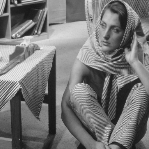
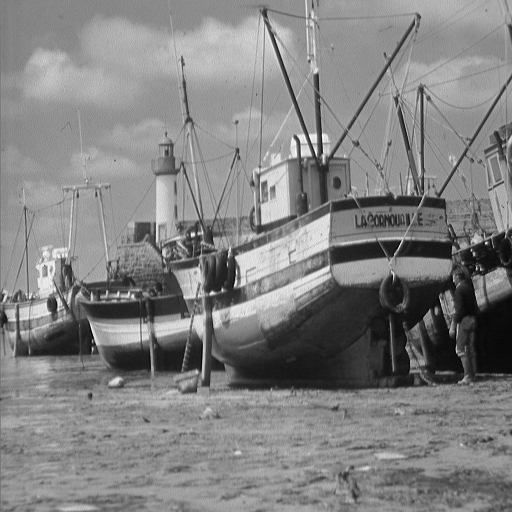
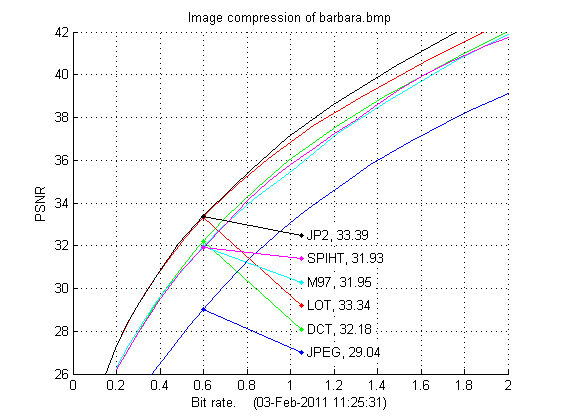
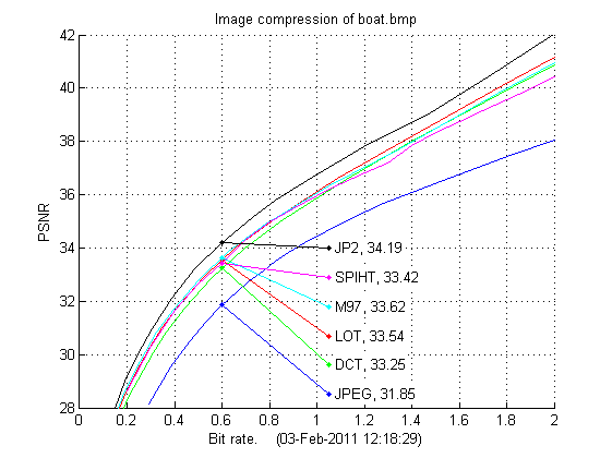
The three test images, lena.bmp, barbara.bmp and boat.bmp, are shown below.
The example in ex01.m compresses Lena using the 8-by-8 2D DCT transform, the 16-by-8 LOT transform and the 9/7 wavelet transform with 3 levels. The results are compared to JPEG and JPEG-2000 (JP2) from Matlab and SPIHT, and are presented in the figures below. The bit rates below are found using Huff06.m, the estimates made by estimateBits.m will be marginally lower.
We note from the lena results below that the compression schemes based on the 9/7 wavelet, (JPEG-2000, SPIHT and M97) compress better than the schemes based on the DCT (JPEG and DCT), the LOT scheme here only compresses marginally better than the DCT scheme. It is also noteworthy that the M97 scheme is a little bit above SPIHT and a little bit below JPEG-2000 even though the entropy coding scheme essentially is much simpler. This shows that the scheme which arrange the quantized coefficients into sequences (as briefly described above and with details in the relativly short m-file myreshape.m) and then do Huffman coding of these sequences, is actually quite effective! The entropy coding in JPEG-2000 is based on the EBCOT scheme (where aritmetic coding is a part) and it is brilliant, advanced and effective. SPIHT uses another effective entropy coding scheme, which also includes arithmetic coding.
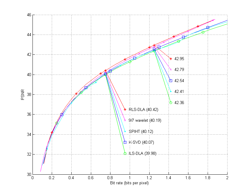
Results for learnt dictionaries i the 9/7 wavelet domain are also presented in the table for the lena test image. Compression is done as described in section 7 right above. We note that K-SVD learnt dictionary performs a little bit better that the dictionary learnt by MOD, and that the dictionary learnt by RLS-DLA is even better, almost as good as JPEG-2000.
| Lena: bit rate | 0.25 | 0.50 | 0.75 | 1.00 | 1.25 | 1.50 | 1.75 | 2.00 |
|---|---|---|---|---|---|---|---|---|
| JPEG | 31.64 | 35.85 | 37.77 | 39.14 | 40.27 | 41.16 | 42.04 | 42.88 |
| DCT | 34.02 | 37.41 | 39.54 | 41.09 | 42.31 | 43.44 | 44.52 | 45.61 |
| LOT | 34.40 | 37.61 | 39.63 | 41.12 | 42.34 | 43.46 | 44.56 | 45.67 |
| SPIHT | 34.78 | 38.11 | 40.12 | 41.40 | 42.41 | 43.26 | 44.48 | 45.31 |
| M97 | 35.08 | 38.29 | 40.19 | 41.61 | 42.79 | 43.90 | 45.00 | 46.13 |
| JP2 | 35.29 | 38.60 | 40.48 | 41.91 | 43.11 | 44.13 | 45.21 | 46.40 |
| Using learnt dictionaries | 0.25 | 0.50 | 0.75 | 1.00 | 1.25 | 1.50 | 1.75 | 2.00 |
| MOD, (D5) | 35.12 | 38.21 | 39.98 | 41.28 | 42.36 | 43.34 | 44.24 | |
| K-SVD, (D7) | 35.13 | 38.26 | 40.07 | 41.41 | 42.54 | 43.56 | 44.52 | |
| RLS-DLA, (D6) | 35.26 | 38.57 | 40.42 | 41.78 | 42.95 | 44.02 | 45.04 |
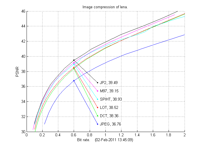
Above is for methods using no dictionaries.
Here are two figures of compression result for the lena test image.
The 9/7 wavelet (M97) and SPITH result should be the same in these two figures.
Below is for dictionaries learnt by MOD (ILS-DLA), K-SVD, and RLS-DLA.
Below are the results for the other two test images presented. Again we see that JPEG-2000 is the best compression scheme. It is also interesting to compare the DCT, LOT and M97 schemes as they all use the same entropy coding, the only difference between these methods is the transform/wavlet used. While the 9/7-wavelet is best on lena both DCT and LOT are better on barbara, where especially LOT compresses well even compared to JPEG-2000. Also on boat LOT is the better transform, but here the 9/7-wavelet is better than DCT. Also for the last two test images the M97 scheme performs almost the same as SPIHT, both are based on the 9/7 wavelet but the entropy coding schemes are very different.
| Barbara: bit rate | 0.25 | 0.50 | 0.75 | 1.00 | 1.25 | 1.50 | 1.75 | 2.00 |
|---|---|---|---|---|---|---|---|---|
| JPEG | . | 27.77 | 30.74 | 33.09 | 34.95 | 36.57 | 37.94 | 39.10 |
| DCT | 27.06 | 30.95 | 33.76 | 36.02 | 37.83 | 39.37 | 40.75 | 42.03 |
| LOT | 28.30 | 32.17 | 34.84 | 36.83 | 38.51 | 39.95 | 41.28 | 42.52 |
| SPIHT | 27.06 | 30.85 | 33.56 | 35.80 | 37.55 | 39.33 | 40.68 | 41.75 |
| M97 | 27.25 | 30.84 | 33.46 | 35.45 | 37.47 | 39.09 | 40.58 | 41.88 |
| JP2 | 28.40 | 32.24 | 34.89 | 37.18 | 38.92 | 40.50 | 41.90 | 43.13 |
| Boat: bit rate | 0.25 | 0.50 | 0.75 | 1.00 | 1.25 | 1.50 | 1.75 | 2.00 |
|---|---|---|---|---|---|---|---|---|
| JPEG | . | 30.90 | 32.99 | 34.46 | 35.54 | 36.44 | 37.25 | 38.05 |
| DCT | 29.13 | 32.33 | 34.37 | 35.89 | 37.23 | 38.47 | 39.67 | 40.87 |
| LOT | 29.54 | 32.68 | 34.62 | 36.11 | 37.43 | 38.69 | 39.92 | 41.14 |
| SPIHT | 29.51 | 32.63 | 34.68 | 35.96 | 36.99 | 38.35 | 39.37 | 40.42 |
| M97 | 29.67 | 32.78 | 34.67 | 36.04 | 37.25 | 38.48 | 39.74 | 40.95 |
| JP2 | 30.11 | 33.32 | 35.27 | 36.74 | 38.04 | 39.20 | 40.58 | 42.01 |
The experiments are done in Matlab.
Some of the functions, i.e. the sparse approximation part when dictionaries are used, are partly implemented in Java,
and for these to work the Java package mpv2
should be installed. It is a collection of all the Java classes used here.
For more details on how to use this package see the
DLE web page.
| mat-files | Text |
|---|---|
| D1, D2,
D3, D4 D5, D6, D7, D8 |
The mat-files that store dictionaries for images. From left to right they were learnt by the
MOD-method, the RLS-DLA, the K-SVD, and a separable version of MOD. No. 1-4 are in pixel domain, and no. 5-8 are in 9/7 wavelet domain. |
| bmp-files | Images |
| barbara.bmp | The Barbara image, 512x512 grayscale image. |
| boat.bmp | The boat image, 512x512 grayscale image. |
| lena.bmp | The Lena image, 512x512 grayscale image. |
| m-files | Text |
| calic.m | CALIC-like lossless coding of an image (integer matrix) |
| compressSPIHT.m | Compress an image (matrix) using SPIHT. (from www.cipr.rpi.edu/research/SPIHT/spiht3.html) |
| estimateBits.m | Estimate bits for coding a cell-array of integer sequences |
| ex01.m | Example 1: compression of an example image (Lena) |
| ex02.m | Example 2: variants of 9/7 wavelet filters |
| getELT.m | Extended Lapped (orthogonal) Transform, ELT, of size 4NxN |
| getLOT.m | Lapped Orthogonal Transform of size 2NxN |
| getwave.m | Get a synthesis transform matrix based on a dyadic wavelet filter bank |
| imageapprox.m | Approximate an image by a sparse approximation, and it may also compress into a bit stream. |
| imagerestore.m | Restore an image from approximation (or compressed bit stream) made by imageapprox. |
| mycol2im.m | Rearrange matrix columns into image blocks. |
| myilwt2.m | My variant of ilwt2(..), use as ilwt2 with Lifting |
| myim2col.m | Rearrange image blocks into columns. |
| myimadjust.m | Trim or extend image, height and width have given factor. |
| mylwt2.m | My variant of lwt2(..), use as lwt2 with Lifting |
| mypred.m | Prediction in matrix (image) into cell array, or inverse. |
| myreshape.m | Reshape between matrix and cell array of sequences. |
| uniquant.m | Uniform scalar quantization (or inverse quantization) with threshold |
| zip-files | Text |
| comp.zip | The files for entropy coding, including Huff06. Content is listed in comp.pdf |
| Last update: July 2, 2014. Karl Skretting | Visit my home page. |