

Faults, strain, and fault facies
Note: This page describes previous research at CIPR (2004-2008). At the University of Stavanger, we are conducting research on related topics
How do faults form and grow? How do faults influence fluid flow? How should we model faults and their deformation?
From 2004 to 2008 I worked in a project called Fault Facies (Center for Integrated Petroleum Research, CIPR). The aim of this project was to develop a methodology to realistically include faults and their deformation in reservoir models.
In conventional reservoir models, faults are included as planes with distinct transmissibility. However in reality, faults are volumes with complex facies distribution and permeability structure.
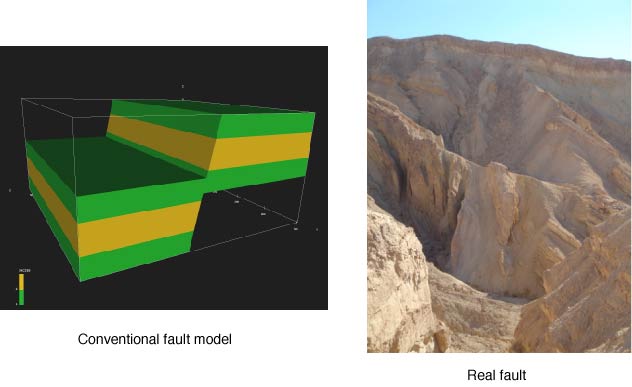
To bridge the gap between model and reality, we need to include faults as volumes in reservoir models. These volumes contain "fault facies" which are rock bodies that have been influenced by faulting. In a manner similar to how reservoir models are populated with sedimentary facies, we want to populate fault volumes (i.e. fault grids) with fault facies.
The methodology is based on the assumption that fault facies are linked to lithology through strain. Within a fault zone, the distribution of fault facies is a function of i. the distribution of host rock materials and ii. strain. These in turn are functions of the kinematics in the fault zone.
My job was to develop tools to predict displacement/strain in faulted reservoirs. These tools should be efficient enough to be included in a standard reservoir model. Our group developed: (i) an inverse modeling program to compute strain from displacement data, (ii) a simple but versatile algorithm to compute strain within the reservoir modeling workflow, and (iii) a more elaborate kinematic model to compute strain in fault-related-fold models. Parallel to these efforts, we also modeled mechanically the evolution of fault zones.
General inverse strain modeling
Displacement data can be used to invert for the best-fit strain tensor. Richard Allmendinger and I implemented the computer program SSPX (Cardozo and Allmendinger, 2009). SSPX is a full-fledged inverse modeling program to calculate best fitting strain tensors given displacement or velocity vectors at a minimum of three points in 2D or four points in 3D. If more than three points in 2D or four points in 3D are available, SSPX uses the extra information to assess the uncertainties in the assumption that the strain in the region encompassed by the points is homogeneous.
SSPX can be used to compute the 2D and 3D strain of discrete element models (DEM) and analogue experiments, strain rates from Geographical Positioning System (GPS) data, or the strain of reservoir modeling grids with nodal displacement data.
A simple algorithm to compute strain in reservoir models
Per Røe and Harald Soleng at The Norwegian Computing Center developed an algorithm to compute strain in faulted reservoir models using the software Havana. The algorithm is based on a simple displacement formula and a volumetric strain computation in the grid's deformed configuration (Cardozo et al., 2008). The algorithm works on corner point grids and is fast. It can easily be introduced in a reservoir modeling workflow that involves stochastic modeling an the building and testing of numerous model realizations. The figure below shows the application of the algorithm to the Emerald field (a tutorial of the RMS software by Roxar). The colors in the grid indicate finite strain (maximum stretch). Red areas are highly strained.

Strain of Emerald model
Harald Soleng has also implemented a simple shear model in Havana for the fault zone. In this model, the fault zone is divided into a discrete number of regions parallel to the fault. In each region, fault slip is allowed to vary linearly or exponentially from a minimum to a maximum value. Adjacent regions have the same fault slip at their boundary, in order to avoid discontinuities. This algorithm gives more flexibility when defining the displacement in the fault zone. However, at the moment the algorithm only works in grids with just one fault.
A strain inverse modeling strategy such as the one used in SSPX can also be implemented in Havana. In this case, the algorithm would compute the strain at each node, based on the displacement of neighboring nodes within a radius. This can be more demanding, but it would eliminate the need of a regular grid for computation (Cardozo et al., 2008). Thus, eliminating some artifacts that we see with the current algorithm in skewed grids.
Forward modeling of fault related folds
The Havana-strain algorithm does not work in cases in which there are variations of slip along the fault dip direction, such as in fault propagation folding. More elaborate models such as trishear are better in these cases.
I implemented a 3D forward modeling program for fault related folding called Trishear3D. The program is based on trishear for the folding ahead of the fault tip line, and standard parallel/inclined shear algorithms for the folding behind the fault tip line. The geometry and finite strain of 3D fault propagation folds, fault bend folds, rollovers, lateral fault propagation, and combination of these cases can be modeled. The results can be visualized in a 3D plot which can be queried for strain or sliced along any orientation. Geometry and strain can also be displayed in tables that can be exported to reservoir modeling or fracture generation software.
The figure below shows an extensional fault propagation fold made with the program. In this example, fault slip decreases along the fault, from the frontal to the rear side of the model. The dots in the figure are tetrahedrons for finite strain computation. The beds are colored by their strain (maximum stretch). Red areas are highly strained.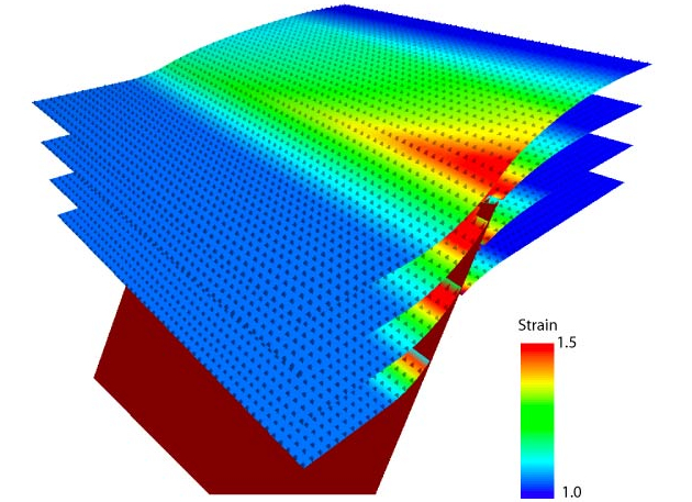
Strain of extensional fault propagation fold made with Trishear3D. More models in this page
Sigurd Aanonsen and I wrote several Matlab scripts to do trishear inverse modeling, i.e. Estimating the trishear parameters that best fit a structure. These scripts rely on several optimization algorithms that significantly speed-up the parameter estimation. We can now conduct 2D and 3D trishear parameter estimation (six or more parameters) in seconds. Optimized trishear inverse modeling has allowed us to address questions such as the uncertainties of the estimated parameters (Cardozo and Aanonsen, 2009).
Mechanical modeling of fault zones
The kinematic models described above are reasonable representations of the geometry and finite strain of fault related folds, but there are no dynamics in these models. The models are based on "ad hoc" displacement or velocity fields.
Parallel to kinematic modeling, we investigated the dynamics of faulting through discrete element, mechanical modeling (DEM). DEM is a discontinuous, mechanical method in which rocks are represented as assemblages of thousands of rigid particles that interact at contacts. Friction and bonding between the particles can be specified. We used a 2D commercial version of the DEM method called PFC2D.
The animation below is a simulation of faulting of soft (orange beds without bonding between particles) and hard (blue bonding between particles) beds. The area is about 15 by 15 m. The superimposed colors are contours of maximum shear strain.