FTCM_interpolate results:FTCM_generate results: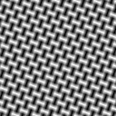
Karl Skretting, University of Stavanger.
| Contents on this page: | Relevant papers and links to other pages: |
|---|---|
|
|
The intention of this page is to present the Frame Texture Classification Method (FTCM) and the Matlab-files that implement the method. In images texture may be regarded as a region where some elements or primitives are repeated and arranged according to a placement rule. In image processing a texture may be analysed, i.e. some appropriate properties can be found, or a texture may be classified, i.e. identify the texture class in a homogeneous region, or an image may be segmented by finding a boundary map between different texture regions. Another use of texture, here a texture model, is to synthesize an artificial texture to be used for example in computer graphics or image compression.
FTCM is based on a tiled floor model which can be used to synthesize a texture. A dictionary, or frame, can be learnt to model an example texture. A test image, a region or a single pixel (with a surrounding neighboring block), can be compared to the texture model represented by the dictionary and the distance to this model is found. This distance is assumed to be proportional to the (negative log) probability for the tested region to belong to the modelled texture class. Classification can be done using several candidate dictionaries (models). Image segmentation based on texture can be done by smoothing the distances to (probabilities for) each candidate texture over the pixels.
This page continues by presenting the tiled floor model, how to learn dictionaries, and how to use these for classification and segmentation. I also intend to present some alternative methods for texture classification. For segmentation smoothing is very important, and this part is actually quite general and can be used also for other kind of segmentation (not based on texture), so it is presented in its own section here. Finally some training and test images are presented, and some results are presented. The results for FTCM are excellent. At the bottom are the Matlab-files listed.
FTCM was first presented in my Ph.D. thesis, and the tiled floor model was first presented in the
EURASIP JASP 2006 paper.
This brief presentation of FTCM is much like in this paper, only shorter.
For more details see the EURASIP JASP 2006 paper. Let us start with some definitions (clarifications):
Classification: Assign a class to a given test exemplar,
which may be a single test vector (belonging to a single pixel or a neighborhood) or the whole test image.
The class for a single pixel may be foreground or background,
for a neighborhood it may be texture 1, texture 2, up to texture M,
or for the whole image it may be "healthy tissue" or "injured tissue".
The output from classification may be a label but more convenient for following processing
is usually an estimated probability for each class, or an estimated distance to each class.
Segmentation: Divide the image into (connected) components where each component usually represents one class.
The main input to segmentation is the (probability or distance) output from classification,
but also additional, i.e. spatial (or temporal), information of the segments is used.
These two parts may be called the data term and the shape term.
labelling: Assign a label to each element (pixel).
The labels are members of a finite set, i.e. integers in range 1 to M or a set of strings (names).
Image classification or segmentation: Image classification of smoothed data may be called
either classification or segmentation, depending on how much importance the authors put into the
implicit "shape information". Since texture property in an image by definition is
a neighborhood and not a pixel property, some smoothing may be done without actually assuming anything
on "shape information" but more smoothing implicit assumes (mainly) larger segments to be present.
FTCM_interpolate.m function.
Here the tile may be defined by a Matlab matrix X, using a 4-by-4 matrix
a 128-by-128 example texture image Y can be defined and displayed
  X = [ 1,0,1,0; 2,0,2,2; 1,0,1,0; 2,2,2,0 ]/2;
  Y = FTCM_interpolate(X, rand(1), rand(1), 0.067, 0.069, pi/9, 1, 128, 128);
  imagesc(Y); colormap(gray); axis equal;
Above a random offset is used, the interpolation grid is rotated 20 degrees (π/9). The resulting image
Y is shown below.
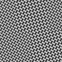
The FTCM_generate.m function was made to generate an image
consisting of blocks from predefined textures.
The following code makes a texture image A, which is shown below.
  A = FTCM_generate([1,2,2,1;1,1,2,2], 128, 64, 30, 0.053);
  figure(1); clf; imagesc(A); colormap(gray); axis equal;
FTCM_interpolate results: |
FTCM_generate results: |
|
|
To go the opposite way, i.e. generate a tiled floor texture model from an example texture may be a
challenging task, especially since real world example textures are not as
regular as a mathematical model and since there is usually also noise (disturbances)
in the image. To learn a tiled floor model directly, finding the tile X and
the parameters to use in FTCM_interpolate from an image Y is still an unsolved problem.
How this model should be used in practical applications has also (to my knowledge) not been considered yet.
An alternative is to learn a dictionary by standard dictionary learning algorithms, and let this
dictionary together with a sparse approximation method be a model of the texture.
For a brief introduction to dictionaries and sparse representation see
the Dictionary Learning Tools web page.
The tiled floor texture model is only used indirectly in FTCM, in the EURASIP JASP 2006 paper
it was shown that this model can be directly transferred to a sparse representation
(or approximation when noise is present) model using a finite dictionary.
The (training and test) vectors are made as image pixels from a local neighborhood around each pixel.
To let a learned dictionary represent a texture is the main idea in FTCM, and
this way both training (learning) and testing can be done by well developed methods.
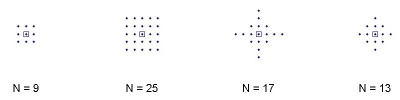
The local neighborhood around a centre pixel can be selected in many ways;
the patches are reshaped into vectors that can be used
as training vectors in a dictionary learning algorithm or
as test vectors in a texture classification algorithm.
The NORSIG 2005 paper
discusses several methods to make these vectors.
The m-file, makevector.m can be used to make these vectors.
Below are some of the possible neighborhoods shown, each dot represent a pixel and the square
represent the center pixel and N is the length of each vector.
 |
Having an example texture it is possible to use a dictionary learning method,
see the Dictionary Learning Tools web page,
to learn a model, i.e. a dictionary, which represents this texture.
I have made a quite general m-file, texdictlearn.m,
that may be used for this purpose. The options are explained in the help text.
Two important parameters are vecMet and the number of dictionary atoms to use K,
these give the dictionary size, NxK.
One way to use this function to make a model (dictionary) to represent one example texture from
the Outex
framework for texture analysis is shown below.
The computational time for learning one dictionary is between 75 and 80 seconds.
  vecMet = 'd';  % as given in makevector.m
  K = 130;       % number of atoms (columns) in the dictionary
  N = size(makevector(ones(19),vecMet,10,10,0),1);   % vecMet == 'd'  ->  N = 13
  n2k = 1000;  % gives 2000*n2k iterations (number of training vectors to process)
  imrange = [-1,1];
  learn_opt = struct('imrange',imrange, 'vecMet',vecMet, 'K',K, ...
     'samet','mexOMP', ...   % alternative 'javaormp' or 'ORMP' (slow)
     'saopt',  struct('tnz',3, 'verbose',0), ...
     'ptc', {{'mtvp','r2avg','traceA','fbB','betamse','d2min','nofr','rcondA','nofo'}}, ...
     'minibatch', repmat([n2k,1],5,1).*[1,20; 2,40; 3,100; 3,200; 2,500], ...
     'lam0', 0.996, 'lam1', 1.1, ...
     'checkrate', 5000, ...
     'dlim', 2.5, 'outlim', 3, ...
     'saveDs', 3, ...   % give 'dictfile' to store dictionary in
     'verbose', 1 );
  fn = '...\Contrib_SS_00000\002\train_01.ras';       % OBS! give correct path here
  dictfile = '...\Contrib_SS_00000\002\Dd130_01.mat'; % OBS! give correct path here
  Ds = texdictlearn('imfile',fn, learn_opt, 'dictfile',dictfile);
Classification of a region (or a single pixel) in a test image is quite simple in FTCM. There should be available one dictionary for each candidate texture, and each dictionary is used to make a sparse representation of the test vectors made from the test image, one test vector for each pixel. For each pixel and each candidate dictionary there will be a representation error, and a pixel by pixel classification (straightforward labelling) of the test image will be to assign each pixel the label corresponding to the dictionary that gave the smallest representation error. This approach used in FTCM will usually give quite large overall error rate, i.e. percentage of wrongly classified pixels for the whole test image. But as texture is not a single pixel property some kind of smoothing should be done and this will reduce error rate considerable.
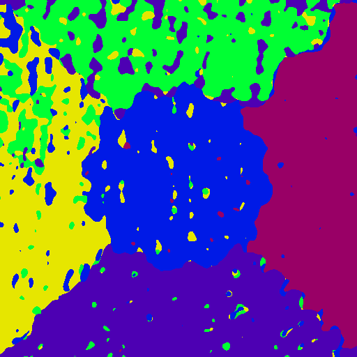
One example using the Outex supervised segmentation test suite Outex_SS_00000
number 23 is presented here, the test image and the ground truth image are shown below.
The matlab file texclassify.m do this classification
and return the 3-dimensional representation error matrix R.
Input to this file is the test image, a cell struct where each element contains
on candidate dictionary, and there are also some optional arguments (ex. ground truth image).
The computational time for classification is a little bit below 40 seconds.
  classify_opt = struct('gt',gtfile, 'verbose',1);  % gtfile is file name (ground truth)
  R = texclassify(testim, Dcell, classify_opt);     % testim may also be file name
  [~, Lmin] = min(R,[],3);                          % Lmin is straightforward labelling
labelling using the representation errors directly (as in the third line above)
usually gives a poor segmentation. The label image, Lmin, will contain
many segments, i.e. connected components, and the error rate will be high.
For the test image below error rate was 65.8% (no smoothing) using dictionaries
learned as the example in section 2.2 above.
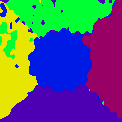
Smoothing the data term R a little bit improves classification result, σ=2 gives error rate 28.3%.
To improve results even more more smoothing (or a smarter segmentation) should be done.
This segmentation step is a general step in image processing and not especially connected to FTCM,
and some possible approaches are presented in the next section.
 |
 |
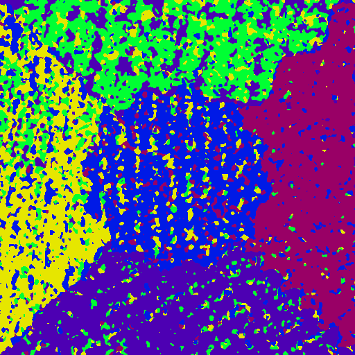 |
| Outex SS test image 23 | Ground truth label image | Results using σ=2, error rate = 28.3% |
Although this part is written in the context of texture segmentations the methods presented are quite general and can be used for image segmentation in general, for example based on color (gray tone), edge detectors or output from other filters. The main idea is that each image pixel should be labelled as belonging to a object or kind (of texture). There may often be restrictions on these objects, like size, for example one pixel sized textures are impossible (to observe), or numbers, for example one background and some few objects, or kind, for example vegetation, buildings or roads, and lakes in an aerial image. For the textures test images each segment should belong to one of the predefined candidate textures, and we also assume that there should not be too many segments in each image (or that segments should not be small).
Segmentation is always based on some observations (here a test image) or data calculated from
the observations. This is the data term (denoted R above,
for an I×J image and M classes R is an I×J×M matrix)
and can be thought of as costs (for assigning a given label to a pixel)
or energy (similar to cost in an energy minimization set-up)
or probabilities (the probability that each pixel belongs to each class).
The matrix R is returned by texclassify.m,
but it can also be made in other ways.
In addition shape information may be used,
and this may be expressed as a shape term, as in section 3.2 below.
Smoothing is an important part of most texture classification and segmentation methods, especially for the filtering method where many variants have been used, see part 2.1 in the IEEE Trans. PAMI 1999 paper by Randen and Husøy and the many references given there. A common setup is a nonlinearity (magnitude, squaring, sigmoid, or logarithm) followed by a Gaussian or rectangular smoothing filter. For FTCM many methods have been used too, see section 6.3.2 and figure 6.6 in my Ph.D thesis for details, but I now think that simple Gaussian filtering (using standard deviation σ in range from 4 to 16) directly on the magnitude (2-norm) of the representation errors will do quite well in most cases. The matlab file LIS_smooth.m do this Gaussian smoothing, resulting labelling for the classification above done with σ=4 (error rate 13.3%) and σ=8 (error rate 6.6%) and σ=16 (error rate 4.6%) are shown below.
 |
 |
 |
| Results using σ=4, error rate = 13.3% |
Results using σ=8, error rate = 6.6% |
Results using σ=16, error rate = 4.6% |
From the results above we see that the overall classification improves (for this particular test image) as the standard deviation σ for the low pass filter increases. We also see the disadvantage that details are smeared out and fine details are completely removed, see for example the border line connected to lower right corner, its wave shape clearly visible for σ=4 but the line is almost straight for σ=16. Also a large value for σ do not necessarily removes small segments or "transition" effects on the border of segments.
Energy minimization is a way to address the fact that image segmentation consists of
at least two terms; a data term derived from the observations and a smoothing term that
comes from assumptions about "smoothness" of the resulting label image.
There may also be other information available which may be taken for granted (like which
classes may be present in the image) or ignored (like number of segments or the probably
size of each segment). The energy minimization set-up defines an objective function
to be minimized; this function depends on the chosen labelling L
(and data R of course) and typically is defined using two terms
E(R,L) = Edata(R,L) + Esmooth(L). |
(3.1) |
Energy minimization is not a new approach to image segmentation, a good and brief presentation is given in the introduction of the IEEE Trans. PAMI 2001 paper Fast Approximate Energy Minimization via Graph Cuts by Y. Boykov et al. They refer to earlier papers by R. Potts (1952), Grimsom (1985), J. Besag (1986), D. Terzopoulos (1986), D. Lee (1988) and more. This work of Boykov et al. is particular interesting for the work presented on this page as I have implemented Matlab functions that depend on the effective (mex-file) Kolmogorov implementations, see the Vision Group at UWO code web page and the Boykov-Kolmogorov algorithm for Max-Flow or Min-Cut problem. The paper by Boykov et al. describes in detail both the swap-move and expand-move used in LIS_swap.m and LIS_expand.m and the newer EMP8_swap.m. These moves (swap and expand) have also been used by others, see the CVPR 2008 paper by Mairal et al. Discriminative Learned Dictionaries for Local Image Analysis, where very good results for texture segmentation are presented.
Since the early 2000s, significant progress has been made in texture image classification and related research areas. For a detailed overview of min-cut/max-flow algorithms, I refer to the 2022 IEEE Transactions on PAMI paper Review of Serial and Parallel Min-Cut/Max-Flow Algorithms for Computer Vision by P. M. Jensen et al., see IEEE Xplore and/or Github. Below, in section 3.3 2025 update on energy minimization, I try to relate (the new Python implementation of) the erode algorithm to their work.
The form of the energy function is of course important, since it measures each labelling and gives a way to say if a labelling is better than another labelling thus defines which shapes are preferred, and since its form is important for how to (approximately) minimize the function. Like Boykov in the 2001 PAMI paper we consider a commonly used form of energy functions which may arise from first-order Markov Random Field models:
E(R,L) = ∑p∈PR(p,L(p)) +
∑p,q∈NV(p,q,L(p),L(q)) |
(3.2) |
p and q are pixels indices, P is
the set of all pixels and N is the set of all pairs of neighboring pixels.
The first term here is the data term and is simply the sum of elements in matrix R,
one element for each pixel, which element is given by the assigned label
(1 ≤ L(p) ≤ M). The second term, the shape term, is more
complicated but essentially of the same form as the data term, the shape term adds
costs given by function V for all neighboring (interacting) pairs of pixels.
One of the more simple, but useful, forms for the V-function is the
Potts model where V(p,q,L(p),L(q))=c for all neighbor pairs
if the pixel labels differ, i.e. L(p) ≠ L(q), else V(⋅)=0.
As neighboring pairs usually only the 4-pixel-neighborhood or the 8-pixel-neighborhood is used.
But even for this simple form of energy function it is in general an NP-hard problem to minimize it.
Here we suggest to replace the parameter (constant) c
in function V(⋅) by another parameter λ which gives the
relative importance of the shape term to the data term. The purpose of this
is to make it easier to set an appropriate value for the parameter for a specific kind of problems.
To do this the data term should be scaled (and translated) such that the minimum labelling,
i.e. Lmin as given in Matlab code in section 2.3 above, gives a value 0
and the corresponding maximum labelling Lmax gives a value 1.
Thus we will have for the scaled data term 0 ≤ Edata(R,L) ≤ 1.
Also, the constant c used in Potts model is fixed, we set it to be λ over "the total number of 4-neighborhood pairs in the image".
This way the smoothing term in equation 3.1 can be written as
λ Esmooth(L) where 0 ≤ Esmooth(R,L) ≤ 1.
The smoothing term may now be seen simply as a cost proportional to the total length of
edges (borders) in the label image scaled such that no edges, i.e. all pixels assigned the same label,
gives Esmooth(L)=0, and maximal number of edges gives Esmooth(L)=1.
The smoothing term λ Esmooth(L) for a checker board labelling where each square has side length λ will be approximately 1, i.e. the same as the maximal data cost.
An 8-pixel-neighborhood can be used instead of a 4-pixel-neighborhood in the Potts model,
this was used by Mairal et al. in the CVPR 2008 paper. Here we also suggest to make
a minor adaptation to the Potts model; giving the pairs that only share a corner point a lower (factor b < 1) cost than the pairs that share a pixel edge,
motivated by the fact that these pixels centres are farther apart;
to weight the 4 corner pixels relative to the distance gives that
b=½√2≈0.7 may be suitable. This value will also give a
45 degrees slanted border line the same cost as a horizontal (or vertical) border line
with the same length. Setting b=0 will be like using only the 4-pixel-neighborhood,
and we see that any value of b in range from 0 to 0.7
(or perhaps even 1 as in a true 8-pixel-neighborhood Potts model) will be sensible.
Let E4(L) be the smoothing cost associated to a 4-pixel-neighborhood in the Potts model, and let E8(L) be the additional terms for an 8-pixel-neighborhood,
(0 ≤ E4(L) ≤ 1) and (0 ≤ E8(L) ≤ b),
the suggested energy function for the slightly modified Potts model is
E(R,L) = Edata(R,L) + λ(E4(L)+E8(L)). |
(3.3) |
A Matlab file, LIS_cost.m or the newer version EMP8_cost.m, can be used to calculate the energy (cost) for a given labelling and data term, default value for b is 0.7.
Using this (old) function the energies (cost) for the examples shown above are:
  Labelling       Edata     lambda      E4        E8     E(R,L)  error rate
    Ltrue --> E = 0.29160 +  2.00*(0.00481 + 0.00493) = 0.31107, err.  0.000%
     Lmin --> E = 0.00000 +  2.00*(0.71573 + 0.50354) = 2.43852, err. 65.830%
      Lg2 --> E = 0.23939 +  2.00*(0.09709 + 0.09388) = 0.62134, err. 28.268%
      Lg4 --> E = 0.27487 +  2.00*(0.02778 + 0.02746) = 0.38534, err. 13.349%
      Lg8 --> E = 0.28768 +  2.00*(0.00925 + 0.00902) = 0.32422, err.  6.600%
     Lg16 --> E = 0.29423 +  2.00*(0.00559 + 0.00529) = 0.31600, err.  4.641%
     Lg24 --> E = 0.29709 +  2.00*(0.00481 + 0.00451) = 0.31573, err.  4.399%
     Lg32 --> E = 0.29978 +  2.00*(0.00442 + 0.00415) = 0.31693, err.  4.728%
The results for Gaussian smoothing using σ=24 and
σ=32 is also added it the table above.
This shows that the smoothing energy (border cost) decreases as σ increases,
while the data energy increases.
The total energy first decreases, then reaches a minimum and then increases as σ increases.
Since we here have the true labelling available an error rate can be found for
each labelling, and we note that the error rate seems too be best when the
energy function is small. This indicates that the energy function is reasonable.
Above, no attempt has been made to minimize the objective function in equation 3.3.
It has only been used to estimate "the quality" of the Gaussian smoothing function.
We might think that this simple use of the energy function will be useful
to find a good value for σ to use in the Gaussian smoothing, but this is an illusion
as we only replace one parameter σ by another λ and the first
one is just as easy to interpret as the second one.
These two moves are described in the PAMI 2001 paper by Boykov et al. and they can both be effectively implemented by a max-flow min-cut algorithm. They work under some (mild) restrictions for the cost function, see Boykov et al., but the important thing here is that the objective function as expressed in equation 3.3 is fine. The α-β-swap considers pixels that are labelled α or β and then allows each of these to be relabelled to either α or β. The α-expansion move considers all pixels and each pixel may be relabelled to α or it can retain its original label. Both moves are optimal with regard to the objective function and the inherent restrictions of the move. A third move, α-expansion β-shrink, was proposed by Schmidt and Alahari 2011. This is like α-expansion but it also allows a pixel to be relabelled from α to β. For a two label image the α-β-swap move will find the optimal labelling in one move. For multi label images the moves should be done in a loop stepping through all label pairs for α and β (or all labels for α) until no improvements (relabelling) can be achieved. For multi label images the minimization problem (equation 3.3) is NP-hard so the procedure above is not guaranteed to find the optimal labelling.
The Matlab implementations (for two dimensional images) in LIS_expand.m and LIS_swap.m mainly follow the description of Boykov et al. with one exception.
I found that each move could be "too greedy" such that it relabelled to many pixels (for example all pixels to α), and that slowing down the updating "speed" could improve the final results. This can be done by introducing a parameter borderWidth that restricts the number of pixels under consideration in each move, only pixels within a (small) distance from the label regions borders are allowed to be relabelled.
Another way is to slightly modify the data matrix used in the move, i.e. slightly reduce the cost associated with the current labelling, this can be done by a parameter brems.
The newer implementation in EMP8_swap.m may be easier to use and may give better results.
The results for the test image used above are now better than for Gaussian smoothing. The labelling after Gaussian smoothing with σ=2 was used as initial labelling. Since the order for the label pairs are random in my implementation it may return slightly different results each time the function is executed. On this particular test image the moves worked well also without slowing down the "updating speed". We observe only marginal differences (on this test image) between using swap and extend moves; they both find a lower value for the objective function than the value for the ground truth labelling. The label images below are larger than the ones above to make it possible to notice the details, but the differences between these two images are more difficult to notice (actually only 47 pixels are different here).
  labelling        Edata     lambda      E4        E8     E(R,L)  error rate
    Ltrue --> E = 0.29160 +  2.00*(0.00481 + 0.00493) = 0.31107, err.  0.000%
    Lswap --> E = 0.28605 +  2.00*(0.00482 + 0.00464) = 0.30497, err.  1.358%
  Lexpand --> E = 0.28607 +  2.00*(0.00482 + 0.00463) = 0.30496, err.  1.360%
Click on the icon below to see large label image.
|
|
Results using swap, error rate = 1.4% |
|
Results using expand, error rate = 1.4% |
|
Results using erode, error rate = 1.2% |
|
|
Results using erode + icm, error rate = 1.3% |
|
Results using erode + swap, error rate = 1.4% |
|
Results using erode + swap + icm, error rate = 1.4% |
Here the previous version LIS_erode.m is described, but the newer version EMP8_erode.m is basically similar. I have tried to describe how to use the new version in its help text, and the help text of EMP8_argin.m describes the input arguments, and the help text of EMP8_cost.m describes the small addition done in the cost function.
The results for the test image above are as good as we can hope for,
but for other test images results are not so good even though they usually are
better than Gaussian smoothing. We have developed another algorithm
that also use the cost function in equation 3.3 but in a more indirect way
than the swap and expand functions above. The expected smoothness (or shape)
information is directly used in the algorithm by
1) always erode segments smaller than a limit (10 pixels), also if
the value of the objective function increases when it is removed, and
2) never erode a segment larger than a limit (10000 pixels), not even if
the value of the objective function decreases when it is removed, and
3) a segment larger than first limit and smaller than second limit is eroded
only if this causes a decrease in the value of the objective function.
A brief description of the algorithm follows.
The algorithm start by dividing the input labelling into connected components (segments) and orders these in increasing order. Starting with the smallest segment each segment is "eroded" one by one. This is done by allowing the surrounding segments to relabel a border pixel to its own label, and this relabelling is done in an order given by the objective function such that pixels that decrease its value more are relabelled before pixels that decrease its value less, and pixels that increase its value less are relabelled before pixels that increase its value more. This way the segment under consideration is eroded. Typically when a segment is eroded the first pixels relabelled will cause an increase in the value of the objective function and the last pixels will cause a decrease in its value. In the end there may be an increase or a decrease of its value, and, assuming that the segment size is between the two limits, this value decides whether the erosion should be accepted or the segment restored. A fast implementation of this algorithm is possible using effective implementations for finding connected components in the label image and for the priority queues needed for both the segments and the pixels within each segment. Also note that to find the change in the objective function when relabelling only one pixel can be done very fast.
Using LIS_erode.m the value of the objective function is decreased, for λ=2 and initial labelling from Gaussian smoothing (σ=2) it is decreased from 0.62134 to 0.31095, which is actually a little bit lower than its value for the true labelling, 0.31107. But we note that both swap and expand achieve even lower values for the objective function. When it comes to the error rate erode does marginally better (in this example) with an error rate at 1.247% (swap: 1.358%), this is mainly because erode does not leave small segments on the borders between the larger (true) segments, it only has five segments in the final labelling. On the other hand the border lines are not as smooth as they should be, as clearly can be seen on the figure behind the icon above. An option is to do Iterated Conditional Modes (ICM), see Besag 1986 paper, after erode and thus reduce the value for the objective function, and hopefully also straighten the border lines. This is partly achieved, but it also introduces some small segments at border lines (ex. in the lower part of the green segment), see above.
If we do not like these border lines, one way to (possible) improve, or at least to improve the value of the objective function is to do swap moves on pixels near each border line. We can also do an ICM step after the swap moves; this might relabel pixels where border lines meet each other. Both alternatives were tried and results are shown in table below, and behind icons above. We note that the swap moves are able to decrease both the data term and the smoothing term of the objective function when they are done after the erode function. The results are now very similar to if swap or expand method (loops until convergence) were done directly on the labelling after Gaussian smoothing (σ=2). One obvious advantage of the erode algorithm is the computational time which is less than 0.5 seconds, or a little bit more than 1 second it swap moves are included.
  labelling        Edata     lambda      E4        E8     E(R,L)  error rate
    Ltrue --> E = 0.29160 +  2.00*(0.00481 + 0.00493) = 0.31107, err.  0.000%
 Lerode00 --> E = 0.29058 +  2.00*(0.00509 + 0.00509) = 0.31095, err.  1.247%
 Lerode01 --> E = 0.28874 +  2.00*(0.00503 + 0.00490) = 0.30860, err.  1.276%
 Lerode10 --> E = 0.28648 +  2.00*(0.00477 + 0.00462) = 0.30526, err.  1.371%
 Lerode11 --> E = 0.28629 +  2.00*(0.00479 + 0.00461) = 0.30510, err.  1.357%
       ||-> indicate if ICM is done near the borders after erode (and swap)
       |-> indicate if swap is done near the borders after erode
The obvious way to get rid of the problem with the small segments on the border lines is to increase the weight of the smoothing term, i.e. increase λ. This helps; using λ=3 gives fewer small segments but it also straighten the meandering border lines that should be between segments. The table below shows that the smoothing term is lower after swap and expand than for the true labelling. For this particular experiment (λ=3) swap is the better method.
  labelling        Edata     lambda      E4        E8     E(R,L)  error rate
    Ltrue --> E = 0.29160 +  3.00*(0.00481 + 0.00493) = 0.32081, err.  0.000%
    Lswap --> E = 0.28731 +  3.00*(0.00458 + 0.00435) = 0.31410, err.  1.633%
  Lexpand --> E = 0.28765 +  3.00*(0.00451 + 0.00433) = 0.31416, err.  1.801%
 Lerode00 --> E = 0.29115 +  3.00*(0.00502 + 0.00508) = 0.32144, err.  1.833%
 Lerode11 --> E = 0.28739 +  3.00*(0.00462 + 0.00446) = 0.31465, err.  2.185%
The purpose of the example above was not to conclude on which method
is the best one for image segmentation but simply to illustrate some properties
for each of them. Larger data sets are tried in the examples in section 5,
and the methods still performs quite equal to each other, but for these examples
erode performs on overall a little bit better, and is faster than the other methods.
Anyway, the most important issue is how well classification is done, see sections 2 and 4.
Classification gives the important data matrix R used in the objective function.
The possibilities here are vast: Different methods (each with many possible parameters),
FTCM; different dictionary parameters (K, vecMet, sparseness,
dictionary learning methods and sparse approximation algorithms),
and discriminative dictionaries as Mairal et al. 2008.
The second most important issue is, in my opinion, the choice of objective function,
and if its form is as in equation 3.3 the parameters λ and b.
Only at third place I will put the choice of algorithm to minimize the energy function,
the three methods used above performs quite equal to each other. We also note
that the true labelling is not the labelling that minimizes the objective function.
Since the early 2000s, significant progress has been made in texture image classification and related research areas. For a detailed overview of min-cut/max-flow algorithms, I refer to the 2022 IEEE Transactions on PAMI paper Review of Serial and Parallel Min-Cut/Max-Flow Algorithms for Computer Vision by P. M. Jensen et al., see IEEE Xplore and/or Github. In addition to presenting various algorithms and their variants, the authors provide a comprehensive performance comparison and offer recommendations on which algorithm is best suited for different problem families.
First, it is important to note that the problems addressed by the min-cut/max-flow algorithms — and the erode algorithm presented in our ICIAR 2014 paper and in Section 3.2.3 of this document — are fundamentally different. Min-cut/max-flow algorithms typically solve the maximum flow problem, or its dual, the minimum cut problem, on a directed graph. These algorithms are widely used in computer vision tasks that can be formulated as binary energy minimization problems, such as the one described in Equation (1) of Jensen’s SCIA paper. In such cases, the problem is reformulated as a graph, solved, and the solution is transformed back to the optimal solution for the binary labeling problems. For more general labeling problems — where the number of possible labels is larger than two — solutions can be approximated using a sequence of swap or expansion moves, in each step either a better labeling is found or the labeling is not changed. However, the final resulting labeling is not guaranteed to be globally optimal.
On the other hand, the erode algorithm begins with an initial labeling — typically one that minimizes only the energy function data term, or a mildly low-pass filtered version of the data term. This initial labeling should consist of many small segments, defined as 4-neighborhood connected components. In simplified terms, the erode algorithm places these segments into a priority queue, with the smallest segments at the top. The algorithm then processes the top segment by relabeling its pixels to match the label of a neighboring segment. This causes the segment to be eroded from its boundary toward the center. If this relabeling reduces the value of the energy function, the change is accepted and the priority queue is updated. If not, the original labeling is retained and the segment is simply removed from the queue. The algorithm continues by eroding the next segment in the queue. In this way, the erode algorithm gradually improves the labeling step by step. Note that the erode algorithm operates directly on the energy function as defined in Equation (3.2) on this page. It is important that the initial labeling includes pixels assigned to all relevant classes. Also, the current Python implementation is not as flexible for the smoothing-term as the mex-file implementation, I hope to add more flexibility also for the Python implementation in 2025. In 2026 I hope to expand the Python implementation of the erode function to also handle 3D image segmentation problems.
The results presented on this page are primarily based on work done in MATLAB over ten years ago. The max-flow algorithm implemented by Boykov and Kolmogorov was used to solve each swap and expansion move as required. The results varied slightly depending on the strategy used to select the moves: using mainly swap moves resulted in many smaller subproblems, while relying more on expansion moves led to larger subproblems and fewer steps. Despite these differences, both approaches produced similar final labelings and comparable values for the energy function. The labeling is influenced somewhat by the strategy used to choose the moves, but not by the specific max-flow algorithm employed to solve each subproblem. Therefore, the differences among various max-flow algorithms are not reflected in the final result, but rather in performance metrics such as execution time, memory usage, problem size, and representation. This performance aspect is the focus of Jensen’s SCIA paper.
I do not believe that recent developments in max-flow algorithms will affect the results presented on this page. Similarly, whether the erode algorithm is implemented in Python or as a MATLAB mex-file should not influence the outcomes. Therefore, the results from 10–15 years ago, as shown here, should still be valid. The erode algorithm remains relevant primarily for multi-label 2D image segmentation problems that can be formulated as minimizing an energy function, such as the one defined in Equation (3.1) on this page. For binary segmentation, the max-flow algorithm typically finds the minimum of the energy function and likely also the best labeling.
In the specific class of problems discussed here, a ground-truth labeling is provided. Interestingly, the energy value for this true labeling is not the minimum, indicating that minimizing the energy function does not necessarily yield the correct labeling. Moreover, as the results on this page demonstrate, the labeling produced by the erode algorithm is often closer to the true labeling than the one obtained using swap and expansion moves — even though the latter often achieves a lower energy value.
The results presented on the ICIAR result page show that, for the 12 specific test images used in the ICIAR 2014 paper, image segmentation using the mex-file implementation of the erode algorithm was 50 to 100 times faster than using swap moves with the max-flow algorithm implemented in C by Boykov and Kolmogorov. However, the graphs were generated using my own MATLAB-code, which may have contributed to some of this difference—possibly accounting for up to half of the execution time.
Table 2 in Jensen’s SCIA paper compares time performance of various max-flow algorithms across different problems. It shows that, for 3D segmentation and texture problems, alternative max-flow algorithms can be 2 to 5 times faster than the MBK (Modified Boykov-Kolmogorov) algorithm. For example, the problem labeled texture‑OLF‑D103 (Brodatz?) with a size of 43K nodes has an execution time of 92 ms using the implementation HPF‑H‑L.
Assuming 20 swap moves until convergence for the 5-label problems on the ICIAR result page — many of which use Brodatz textures of similar size (62K pixels, resulting in 20 swap problems each with 20–30K nodes) — we should expect to solve these problems in less than 2 seconds using HPF‑H‑L. This is slightly below the average time for swap moves reported on the ICIAR result page, which is 2.5 seconds.
The Python implementation of erode function, accelerated using Numba, achieves performance comparable to the mex-file version. All of this suggests that the erode function remains a strong choice for texture image segmentation. Even if the performance gap has narrowed by a factor of 10, it should still be 5–10 times faster than newer implementations using swap and expansion moves.
Could perhaps be used for texture classification too?
Could perhaps be included here?
The details on the result page show that energy minimization is considerable better at segmentation than Gaussian smoothing. For this set of test images Erode is better at segmentation than Expand and Swap, even though Expand and Swap generally achieve a better (lower) value for the objective function.
Test image number 23 from Outex supervised segmentation test suite Outex_SS_00000 is used as an example above. This is one of 100 similar test images, i.e. the same ground truth image but different textures. FTCM is used on all 100 test images and segmentation results are briefly presented below.
Dictionaries as described in section 2 and 3 above, i.e. the size is 13×120,
are learned for all textures used in the 100 test images given in
the Outex supervised segmentation test suite. Here λ=2 is used.
They all have a true labeling as presented in section 2.3
where also test image number 23 is shown. In the table below the average results,
and for some particular (and difficult) test images, are presented as error rate in percent.
Dictionary 13×120 |
Average 0-99 | #22 |
#31 | #32 | #84 |
|---|---|---|---|---|---|
Gaussian smoothing σ=8 | 6.4 | ||||
| Swap | 2.52 | ||||
| Expand | 2.63 | ||||
| Erode | 3.15 |
For image 32 the values of the objective function are:
E(Ltrue)=0.26146, E(Lswap)=0.25698,
E(Lexpand)=0.25704, and E(Lerode)=0.25978.
It is also so that because of random elements in these function it may happen that
Expand do as well as Swap (1 percent error) or Swap do as Expand (10 percent error).
We may also want to see more than the average (mean) for these 100 test images, below is a table with several properties for each of the same methods as above.
 vecMet = d, N = 13, K = 120, lambda = 2.0, 100 test images
       min  median   mean    max    std     #>20  #>10   #>5   #>2 #>mean
 Lg8:  2.65   4.87   6.40  22.45   3.84        3    16    49   100     34
 Lsw:  0.97   1.56   2.52  20.86   3.30        1     6     8    24     13
 Lex:  0.96   1.58   2.63  21.12   3.44        1     7     9    25     14
 Ler:  0.96   1.61   3.15  23.61   4.00        2     5    17    31     20
A conclusion is that energy minimization is much better than Gaussian smoothing. For this set of test images Swap and Expand methods are better than Erode.
The process to make a paper presenting the erode-algorithm has been a long one. As a consequence the experiments have been done in many variants, and the results have minor differences from time to time. The first publication was in the ICIAR 2014 conference in Vilamoura, Portugal, see the ICIAR 2014 paper. The same, and some more, results made June 30th 2014 are also presented on my ICIAR result page. They were generated using LIS_erode and other Matlab files that are now replaced by the usually better and more flexible EMP8_erode (and other). The file EMP8_ex5.m can now be used to generate similar (usually a little bit better) but not the same results as on the ICIAR result page.
Since the ICIAR paper was made, an important improvement has been added to the mex-files which cause the interface to change. Thus they were renamed to have prefix EMP8, Energy Minimization using Potts model with 8 neighbors. The change is that it is now possible to include a factor upq to use together with the smoothing cost between pixels p and q, as in equation (2) in the ICIAR 2014 paper. This factor can be included by setting a switch, swUpq=2 or swUpq=3, see help for EMP8_argin.m, to either give a symmetric weight for all pairs in an eight-neighborhood or to calculate this factor based on the difference between the grey levels in the two pixels in the test image.
These changes may improve the results even more. The best results achieved was just below 2 percent error rate, but small changes in data matrix R and the parameters used in the smoothing term may give larger error rate. The results shown below are for one of the best choice of parameters, using K=190, vecMet='g', lambda=4 and erode followed by swap moves in EMP8_ex5.m. The results for the 12 test images are given below:
EMP8_ex5: Outex Contrib SS, vecMet = 'g', N = 17, K = 190, lambda =  4.00, swUpq = 3
                       Ed         lambda  E4       E8           E      error rate %   time
 Test image  1 --> E = 0.10883 +  4.00*(0.00480 + 0.00425) = 0.14502, err.  1.965,   265.2 [ms]
 Test image  2 --> E = 0.18142 +  4.00*(0.00467 + 0.00430) = 0.21729, err.  0.938,   294.2 [ms]
 Test image  3 --> E = 0.30327 +  4.00*(0.00446 + 0.00412) = 0.33761, err.  1.941,   324.5 [ms]
 Test image  4 --> E = 0.34145 +  4.00*(0.00482 + 0.00446) = 0.37861, err.  1.857,   340.3 [ms]
 Test image  5 --> E = 0.24606 +  4.00*(0.00499 + 0.00453) = 0.28413, err.  1.117,   302.1 [ms]
 Test image  6 --> E = 0.18405 +  4.00*(0.00465 + 0.00431) = 0.21987, err.  3.815,  1940.9 [ms]
 Test image  7 --> E = 0.24959 +  4.00*(0.00480 + 0.00450) = 0.28681, err.  2.909,  1995.8 [ms]
 Test image  8 --> E = 0.20246 +  4.00*(0.00382 + 0.00457) = 0.23599, err.  5.975,  1027.7 [ms]
 Test image  9 --> E = 0.30002 +  4.00*(0.00312 + 0.00375) = 0.32749, err.  0.709,   860.4 [ms]
 Test image 10 --> E = 0.24356 +  4.00*(0.00071 + 0.00080) = 0.24963, err.  0.178,    42.6 [ms]
 Test image 11 --> E = 0.19939 +  4.00*(0.00083 + 0.00093) = 0.20642, err.  0.800,   107.9 [ms]
 Test image 12 --> E = 0.35421 +  4.00*(0.00089 + 0.00089) = 0.36134, err.  0.572,    99.9 [ms]
 Average                                                                    1.898
• See the DLE-page for installation of the mpv2 java package used for sparse approximation.
• The mex-files must be compiled from the c-files to become ready for use,
the command to use should be in the beginning of c-file.
See Matlab mex command and perhaps do mex -setup first.
• The MATLAB files are quite old but should still function as they did 10–15 years ago. However, since then, Python has gained significant popularity as a programming language, and many users—students, researchers, or others—may prefer to use Python instead. To accommodate this, some of the EMP8-functions described above have now (as of 2025) been implemented and are available as Python functions, see
py_fun_and_test.zip.
• I hope that I have included all files needed, if you find something missing just send me an e-mail.
| Python-files | Among other files also some EMP8-functions, including erode |
|---|---|
| py_fun_and_test.zip | Pairs of fun*.py and test*.py files. |
| mex-files | The c-files must be compiled to generate mex-files |
| conncomp_mex.c | c-file for connected components in label image. |
| connected_comp.h | header-file for connected components. |
| priority_queue.h | header-file for priority queues. |
| EMP8_common.h | common stuff for Energy Minimization Potts-8 model mex-files. |
| EMP8_cost_mex.c | c-file for cost (energy function evaluation). |
| EMP8_icm_mex.c | c-file for ICM (Iterated conditional modes) algorithm. |
| EMP8_erode_mex.c | c-file for alpha-erode algorithm. |
| EMP8_erode255_mex.c | c-file for alpha-erode on border regions algorithm. |
| m-files | Text |
| conncomp.m | Find (4-neighbors) connected components in 2D grayscale or label image. |
| FTCM_generate.m | Generate predefined texture image from the FTCM texture model, see Sec. 2.1. for an example. |
| FTCM_interpolate.m | Make an image by interpolating on a (floor of) tile(s), see Sec. 2.1. for an example. |
| EMP8_argin.m | Generate and return the input struct used for the other EMP8 functions. |
| EMP8_cost.m | Return (and display) the cost (energy) for a labelled image. |
| EMP8_erode.m | Erode small components and/or border region on label image. |
| EMP8_icm.m | Iterated conditional modes algorithm to smooth a label image. |
| EMP8_swap.m | Do alpha-beta-swap moves on label image using a max-flow-algorithm. |
| EMP8_ex1.m | EM Potts model 8-neighbors, test different setups for erode |
| EMP8_ex2.m | Test EMP8_cost.m and EMP8_icm_mex (script file) |
| EMP8_ex3.m | Test EMP8_swap.m (script file) |
| EMP8_ex4.m | Test EMP8_erode.m og EMP8_swap.m (script file) |
| EMP8_ex5.m | Complete segmentation experiments, FTCM + EM, |
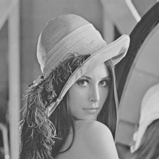
| EMP8_ex7.m | Simple segmentation of lena.bmp. Use no texture information, only White, Gray and Black segments. |
| LIS_getR.m | Get the data term R for test image, matrix R is stored in mat-file. (Obsolete) |
| LIS_maxflow.m | Calls the max-flow (graph-cut) algorithm, i.e use the Kolmogorov implementation in maxflow-v3.01 library. |
| LIS_smooth.m | Find labels after Gaussian smoothing of data cost matrix R. |
| LIS_plotcol.m | Make a color plot (in current figure) of the labelling L. |
| makevector.m | Make (feature) vectors for training or test of textures. |
| texclassify.m | Texture Classification of a test image using dictionaries. |
| texdictlearn.m | Learn a dictionary to represent a texture by a minibatch RLS-DLA variant. |
| teximage.m | Return a (scaled) texture image for training or testing. |
| more m-files | Text |
| java_access.m | Check, and try to establish, access to mpv2 java-package. Some statements in this file should be changed to reflect the catalog structure on your computer, and perhaps also use an m-file like below to return the relevant path. |
| my_matlab_path.m | Return the relevant path for (some of) my matlab catalogs. |
| sparseapprox.m | Returns coefficients in a sparse approximation of each column in a matrix X. |
| Last update: August 15th, 2025. Karl Skretting | Visit my home page. |