
Karl Skretting, University of Stavanger.
The page is still under construction,
the intention is to have some more information on this page.
This page/file is a part of the Texture Classification Tools TCT-page. The conclusion of these experiments are on the bottom of this page.
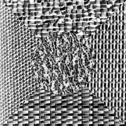
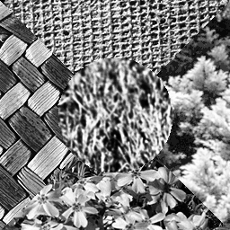
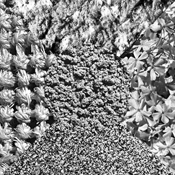
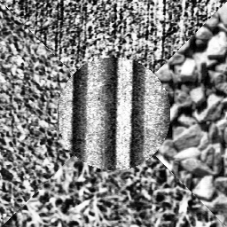
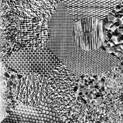
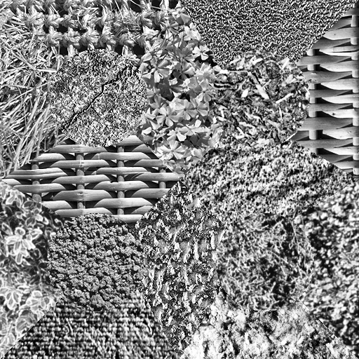
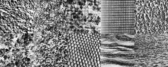
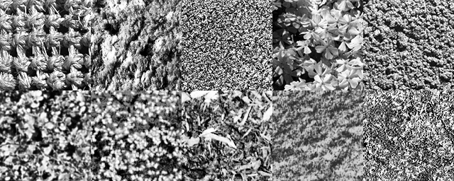
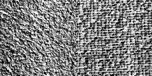
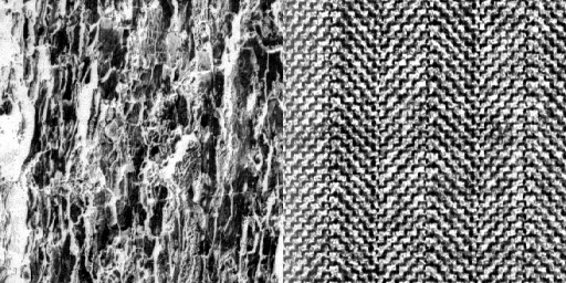
In this section we use Outex contributed supervised segmentation test suite Contrib_SS_00000, the 12 mosaics are used in other works, for example by Randen and Husøy and I have also used the 9 first ones in previous works. The test images are displayed below, click on one to see a larger image. Here the images are numbered from 1 to 12, in the test suite (catalogs, or files) they are numbered from 0 to 11.
|
|
|
|
|
|
|
|
| no. 1 | no. 2 | no. 3 | no. 4 | no. 5 | no. 6 | no. 7 |
 |
 |
 |
 |
 |
| no. 8 | no. 9 | no. 10 | no. 11 | no. 12 |
These test images have been used in some earlier papers, and reported results are listed below,
the numbers are given as percentage of wrongly classified pixels for each of the test images,
average for all 12 images, and average for the 9 first test images in the last column.
• The results from Randen 1999 is the best reported classification for a filtering method
and Gaussian smoothing for each of the test images, i.e. it is not the same method used for all test images.
• From Mäenpää 2000 the result for multi-predicate local binary pattern (MP-LBP)
with predicates one and three (1,3) is presented.
• Skretting 2001 shows the results from his PhD thesis table 6.5 on page 107,
it is FTCM using dictionaries with N=25 (5-by-5 patches) and K=100,
sparseness s=3 and Gaussian smoothing with σ=12 was used.
• Results from Mairal 2008 use discriminative learned dictionaries with
N=144 (12-by-12 patches) and K=128,
sparseness s=4 and Gaussian smoothing with σ=12 was used
for the line indicated by D1. The line indicated by D2 use energy minimization
applying a graph-cut alpha-expansion algorithm based on the Potts model with an 8-neighborhood system.
Mairal 2008 R2 shows results with reconstructive dictionaries (FTCM) and energy minimization,
i.e. Expand, and is the method most comparable to the new results presented here.
• Skretting 2013 is one of the best results presented on this page,
dictionary size 13×200 and λ=2.0, see below.
Method               #1    #2    #3    #4    #5    #6    #7    #8    #9    #10   #11   #12    Av.  Av.1-9
Randen 1999 (best)   7.2  18.9  20.6  16.8  17.2  34.7  41.7  32.3  27.8   0.7   0.2   2.5   18.4   24.1
Mäenpää 2000, MP-LBP 6.7  14.3  10.2   9.1   8.0  15.3  20.7  18.1  21.4   0.4   0.8   5.3   10.9   13.8
Skretting 2001, FTCM 5.9   6.5   9.8   8.9  10.8  21.1  16.3  18.9  20.1    -     -     -      -    13.2
Ojala 2001, LBP      6.0  18.0  12.1   9.7  11.4  17.0  20.7  22.7  19.4   0.3   1.0  10.6   12.4   15.2
Mairal 2008, R2      1.69 36.59  5.49  4.60  4.32 15.50 21.89 11.80 21.88  0.17  0.73  0.37  10.41  13.75
Mairal 2008, D1      1.89 16.38  9.11  3.79  5.10 12.91 11.48 14.77 10.12  0.20  0.41  1.93   7.34   9.51
Mairal 2008, D2      1.61 16.42  4.15  3.67  4.58  9.04  8.80  2.24  2.04  0.17  0.60  0.78   4.51   5.84
Skretting 2013       2.48  2.88  2.23  4.32  2.54  7.72  4.02  2.94  1.90  0.28  1.06  2.10   2.87   3.45
To illustrate the potential and the problems that may occur using FTCM and energy minimization
smoothing as in section 3.2 above, we will look closer on two almost equal cases.
The only difference is that one set of dictionaries uses 200 atoms in each dictionary
while the other set uses 204 atoms. The dictionaries were otherwise learned with
the same parameters, as given in section 2.2 above except that vecMet='g'
giving N=17 and n2k=2000 and of course K=200 or K=204.
During learning training vectors are drawn at random,
so each learning uses different set of training vectors.
Classification, i.e. making the data matrices R, was as in section 2.3.
Using the classification results directly as the data part in the objective function as
in equation 3.3, b=0.7 and λ=2. Initial labelling for
the Swap, Expand and Erode methods was the labelling after
Gaussian smoothing using σ=3.
Below is a table presenting the results.
Method 'g200-2.0'    #1    #2    #3    #4    #5    #6    #7    #8    #9    #10   #11   #12    Av.  Av.1-9
Gaussian sigma=3     6.08 15.42 25.33 21.41 18.20 33.69 37.09 34.94 38.57  2.27  2.44 12.00  20.62  25.64
Gaussian sigma=8     7.29  9.37  9.48  9.24  7.12 21.80 19.72 17.51 15.82  0.28  1.78  4.55  10.33  13.04
Gaussian sigma=12    8.15 10.85 11.41  9.31  6.57 21.25 19.99 16.03 13.02  0.34  2.04  1.91  10.07  12.96
Swap-method          2.56  2.97  2.54  4.14  2.59 10.08  8.76 12.70 11.31  0.28  1.06  2.11   5.09   6.40
Expand-method        2.56  2.84  2.46  4.13  2.58 32.28  9.74 13.80 11.32  0.28  1.06  2.11   7.10   9.08
Erode (swap+ICM)     2.48  2.88  2.23  4.32  2.54  7.72  4.02  2.94  1.90  0.28  1.06  2.10   2.87   3.45
Method 'g204-2.0'    #1    #2    #3    #4    #5    #6    #7    #8    #9    #10   #11   #12    Av.  Av.1-9
Gaussian sigma=3     5.99 14.45 23.98 22.04 16.50 33.84 37.07 36.83 37.26  2.57  2.60 12.33  20.45  25.33
Gaussian sigma=8     7.13  8.93  9.85  9.13  6.22 22.22 19.86 20.94 14.22  0.36  1.87  4.74  10.46  13.17
Gaussian sigma=12    7.73 10.14 11.10  9.33  6.27 21.37 21.14 20.36 12.34  0.32  2.23  2.29  10.38  13.31
Swap-method          2.65  2.56  2.78  4.66  2.57 15.73 11.84 22.19 11.39  0.33  1.12  1.78   6.63   8.49
Expand-method        2.64  2.59  2.78  4.07  2.57 26.93 11.86 22.32 11.28  0.33  1.12  1.78   7.52   9.67
Erode (swap+ICM)     2.69  2.40  2.74  4.27  2.61 14.03  3.46 13.06  1.75  0.33  1.12  1.59   4.17   5.22
There are several observations we can make from these results:
• The results, especially for Gaussian smoothing, are quite similar to each other for the two cases.
• Test image #8 is an exception, here all energy minimization methods happens to classify almost 10 percent
worse for the case with K=204.
• Swap performs on average better than Expand, and Erode considerable better than Swap again.
• The average results for Erode (and K=200) is impressive with only 2.87 percent errors,
all test images, including the difficult ones, are quite well segmented.
• Comparing the average results for Gaussian smoothing with σ=12 we see that
the dictionary setup used here, i.e. N=17 K=200 or K=204,
gives approximately the same classification as the best setup used in my thesis (N=25 K=100)
and is also almost equal as results for the setup used by Mairal.
There are larger differences on the different test images though.
It is more difficult to draw conclusions from these observations (than to observe them).
But I will try to give some brief explanations, based on what I think is reasonable to
conclude from the observed results both the tables above and the details shown below,
and also partly based on my many years of experience with FTCM.
• Different (good) parameter sets for the dictionaries makes only small (on average)
differences on the results after Gaussian smoothing. It seems that the parameter set used here
are better on the more difficult test images and this is an advantage for energy minimization.
• Small difference in the data term, which are exposed after Gaussian smoothing,
may make larger differences after energy minimization.
• Energy minimization is "unstable" as only a marginal change in the
classification results, i.e. data matrix R, may cause a large region of the
test image to be relabelled.
• Swap and Expand usually gives almost exactly the same results, but sometimes a small change
in the minimization algorithm may cause different labelling of a larger region of the test image.
• Swap and Expand found the best values for the objective function,
usually slightly better than the Erode method which again usually was better than the ground truth labelling.
If Swap and Expand gave different results, Expand was usually the better one
with regard to the objective function but Swap with regard to the error rate.
• The main reason for erode to perform better is that erode will not remove a large region
even if that should improve the objective function.
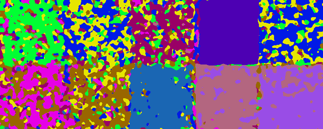
Below we look closer on the difficult test image #8.
The energy function uses λ=2.
Below each figure the different terms of the energy function are written in small green font,
below the test image energy function for true labelling, K=200 data term, is shown,
and below the true labelling the energy function, K=204 data term, is shown.
Since different dictionaries are used the two data terms are only approximately the same.
• Looking at the Gaussian smoothing results we see
that tile 2 (yellow) and tile 5 (blue) are difficult to separate from each other.
For the case with K=200 this is just achieved,
but for the case with K=204 the correct labelling is just missed and
both Swap, Expand and Erode wrongly classify tile 2 as tile 5.
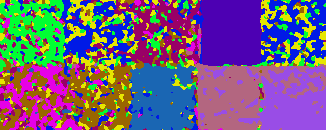
• Another interesting thing is noticed on these examples, tile 6 has many pixels classified
as tile 7, this gives several segments labelled as tile 7 for Gaussian smoothing, but also segments
correctly labelled correctly as 6. Isolating tile 6 would probably show that it is best
(with regard to the energy function) to label it as tile 6, but when we also consider the
neighboring tile it is best (with regard to the energy function) to label it as tile 7.
This is done both by Swap and Extend, but not by Erode since the components labelled as 6
are merged together (or grows together) such that the component get larger enough to be kept
(even if relabelling it to 7 improves energy function).
• This example also illustrate a difference between Swap and Extend,
see the yellow tiles in the second row below.
Extend may often find a marginally better value for the objective function,
but this often imply moving away from the ground truth labelling, and thus Swap as in this example
may have a lower error rate.
|
|
 |
 |
| Test image #8 E = 0.20317 + 2.00*(0.00509 + 0.00709) = 0.22754, er. 0.000% |
K=200 and Gaussian smoothing σ=3E = 0.17809 + 2.00*(0.08532 + 0.08356) = 0.51587, er. 34.943% |
K=200 and Gaussian smoothing σ=12E = 0.20373 + 2.00*(0.01281 + 0.01435) = 0.25805, er. 16.029% |
 |
 |
 |
K=200 and SwapE = 0.20126 + 2.00*(0.00506 + 0.00638) = 0.22413, er. 12.997% |
K=200 and ExpandE = 0.20127 + 2.00*(0.00503 + 0.00638) = 0.22410, er. 13.018% |
K=200 and ErodeE = 0.20058 + 2.00*(0.00565 + 0.00697) = 0.22581, er. 3.389% |
 |
 |
 |
| True labeling for test image #8 E = 0.20376 + 2.00*(0.00509 + 0.00709) = 0.22813, er. 0.000% |
K=204 and Gaussian smoothing σ=3E = 0.17708 + 2.00*(0.08439 + 0.08258) = 0.51103, er. 36.831% |
K=204 and Gaussian smoothing σ=12E = 0.20264 + 2.00*(0.01276 + 0.01428) = 0.25671, er. 20.356% |
 |
 |
 |
K=204 and SwapE = 0.19979 + 2.00*(0.00506 + 0.00640) = 0.22271, er. 22.211% |
K=204 and ExpandE = 0.19975 + 2.00*(0.00505 + 0.00640) = 0.22265, er. 22.319% |
K=204 and ErodeE = 0.20000 + 2.00*(0.00558 + 0.00705) = 0.22525, er. 12.202% |
Apparently not only a marginal change in dictionary parameters and method (for dictionary learning, sparse approximation, or energy minimization) will be important for how well the final segmentation is done, between "failure" and "success". More important, it seems as random factors in these parts also may have an effect, i.e. training vectors are drawn at random during dictionary learning, pairs to swap in each step are processed in random order, the segments to expand are also randomly ordered, and in erode the processing order is random for segments with the same number of pixels, which often occur for small segments. An obvious question to ask is whether the excellent results reported above is just a coincidence or if good results can be expected for all reasonably parameter sets. Another question to ask is the value of parameter λ in the objective function, so far the value of 2 is used all the times, could or should it be smaller or larger. To answer these questions many sets of dictionaries and many values for different parameters should be tried. Some more results are presented in the tables below, here we only show average results for all the 12 test images.
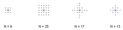 |
The figure above shows some possible different neighborhoods of pixels that are used to make
training and test vectors, and thus give the dictionary parameter N. Those shown
are given by letters 'a', 'b', 'g' or 'd' in makevector.m. Results for
dictionaries for the three rightmost patterns are used in the tables below.
| Dictionary | Gaussian smoothing | Dictionary | Energy minimization, Erode |
|---|
vecMet, N×K |
σ=3 |
σ=8 |
σ=12 |
vecMet, N×K |
λ=1.5 |
λ=2.0 |
λ=2.5 |
λ=3.0 |
mean |
|---|---|---|---|---|---|---|---|---|---|
b, 25×100 |
21.80 |
11.47 |
11.26 |
b, 25×100 |
3.68 |
4.19 |
3.71 |
4.51 |
4.02 |
b, 25×150 |
20.33 |
10.25 |
10.02 |
b, 25×150 |
3.58 |
3.56 |
3.20 |
3.41 |
3.44 |
b, 25×200 |
19.93 |
10.38 |
10.08 |
b, 25×200 |
5.41 |
5.13 |
5.52 |
5.15 |
5.30 |
g, 17×100 |
22.24 |
11.74 |
11.34 |
g, 17×100 |
5.28 |
5.08 |
5.19 |
5.15 |
5.18 |
g, 17×150 |
20.72 |
10.56 |
10.53 |
g, 17×150 |
4.95 |
4.38 |
4.36 |
4.61 |
4.58 |
g, 17×170 |
20.92 |
12.11 |
10.59 |
g, 17×170 |
4.78 |
4.73 |
4.84 |
4.86 |
4.80 |
g, 17×200 |
20.62 |
10.45 |
10.29 |
g, 17×200 |
3.13 |
2.91 |
2.79 |
2.75 |
2.90 |
g, 17×204 |
20.45 |
10.46 |
10.38 |
g, 17×204 |
3.82 |
4.10 |
4.55 |
4.68 |
4.29 |
g, 17×255 |
20.21 |
10.25 |
10.25 |
g, 17×255 |
3.57 |
3.17 |
3.57 |
3.75 |
3.52 |
d, 13×100 |
22.35 |
12.14 |
12.41 |
d, 13×100 |
4.70 |
5.31 |
4.79 |
4.87 |
4.92 |
d, 13×130 |
21.77 |
13.06 |
11.54 |
d, 13×130 |
4.32 |
4.46 |
4.82 |
4.85 |
4.61 |
d, 13×150 |
21.75 |
11.48 |
11.51 |
d, 13×150 |
5.15 |
4.78 |
5.39 |
5.36 |
5.17 |
d, 13×200 |
21.18 |
10.69 |
10.30 |
d, 13×200 |
3.25 |
2.86 |
3.28 |
3.44 |
3.21 |
d, 13×260 |
20.99 |
10.12 |
9.87 |
d, 13×260 |
3.15 |
2.92 |
2.92 |
3.36 |
3.09 |
mean |
21.16 |
11.15 |
10.78 |
mean |
4.25 |
4.19 |
4.26 |
4.38 |
4.27 |
| Dictionary | Energy minimization, Swap | Dictionary | Energy minimization, Expand |
|---|
x, N×K |
λ=1.5 |
λ=2.0 |
λ=2.5 |
λ=3.0 |
mean |
x, N×K |
λ=1.5 |
λ=2.0 |
λ=2.5 |
λ=3.0 |
mean |
|---|---|---|---|---|---|---|---|---|---|---|---|
b, 25×200 |
6.48 |
6.32 |
6.13 |
8.31 |
6.81 |
b, 25×200 |
6.79 |
7.91 |
7.94 |
12.42 |
8.77 |
g, 17×200 |
4.20 |
5.12 |
5.48 |
8.45 |
5.81 |
g, 17×200 |
4.57 |
7.03 |
8.62 |
10.95 |
7.79 |
g, 17×255 |
4.65 |
6.49 |
6.80 |
7.60 |
6.38 |
g, 17×255 |
5.19 |
7.96 |
9.24 |
10.58 |
8.24 |
d, 13×200 |
4.35 |
6.76 |
6.93 |
8.76 |
6.70 |
d, 13×200 |
4.40 |
9.47 |
10.46 |
11.28 |
8.90 |
Some observations:
• For Erode a value of λ in range from 1.5 to 2.5 (or 3.0) is ok,
the results does not depend very much on λ within this range.
• The tables for Swap and Expand
show that a low value (1.5) of λ is the better one,
neighboring segments are more likely to be joined as λ increases.
• Swap and Expand for the reconstructive dictionaries here performs comparable to
the discriminative dictionaries with energy minimization smoothing as used by Mairal in 2008.
• There are some, probably mainly random, differences between each set of learned dictionaries, some sets perform very well while others perform just well.
• It is not possible to say which vecMet is best,
I have a weak favourite in 'g' giving N=17.
• It also seems as large dictionaries K≥200 is the better ones
(except for the 'b' type, N=25).
• FTCM seems to be able to segment these difficult test images quite well,
with an error rate down to 10 percent using Gaussian smoothing.
Minor improvements have been presented since FTCM was presented more than 10 years ago,
the idea with discriminative dictionaries press error rate a little bit below 10 percent.
• Energy minimization can halve the error rate compared to Gaussian smoothing.
The Expand method is the one that best minimize the objective function, but the Swap method is
very close. Achieved error rates with Expand are reported below 5 percent by Mairal using
discriminative dictionaries, and for the best dictionary sets shown above with
reconstructive dictionaries.
• Energy minimization is unstable; a small deterioration in the data term may
cause a large increase in the error rate. This "weakness" is observed both in the
results by Mairal and the results shown above.
• The newly proposed energy minimization scheme, Erode, often avoid this
stability-"weakness" mainly by including an upper limit for when segments
should be considered to be removed, but essential it is still unstable.
The results are excellent, better than Expand, and for the best dictionary sets
the eror rate is below 3 percent!.
| Last update: July 1, 2014. Karl Skretting | TCT-page. |